Section 1 Melanin binding pilot peptide array
library(seqinr)
library(Peptides)
library(stringr)
library(protr)
library(plyr)
library(randomForest)
library(ggplot2)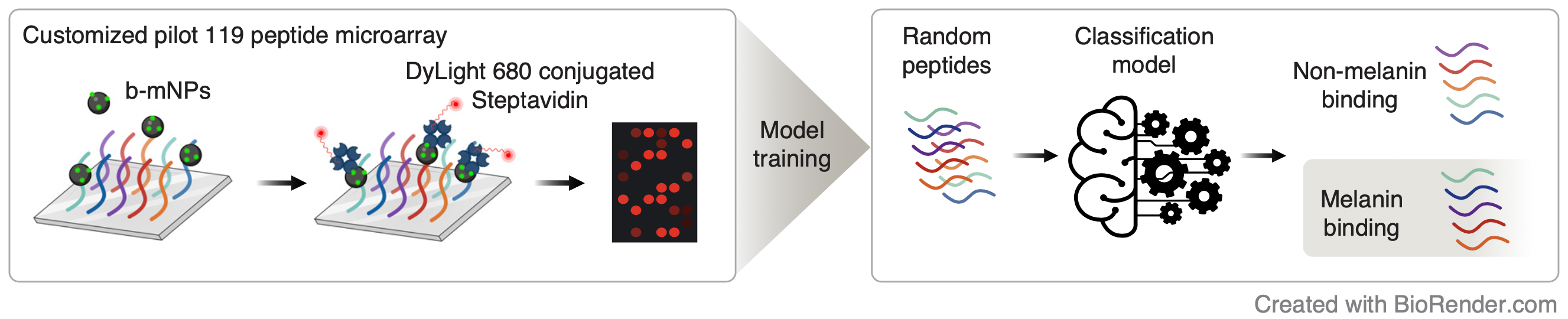
1.2 Generating ML input
# --------------
# Peptides_2.4.4
# --------------
# read in fasta file
peptides <- read.fasta("./other_data/mb_pilot_peptide_array.fasta", seqtype = "AA", as.string = TRUE, set.attributes = FALSE)
# Molecular weight
weights <- as.matrix(sapply(peptides, function(x) mw(x, monoisotopic = FALSE)))
colnames(weights) <- "weight"
# Amino acid composition
aa.comp <- sapply(peptides, function(x) aaComp(x))
aa.comp.matrix <- t(sapply(aa.comp, function(x) x[, "Mole%"]))
# Isoelectric point
pI.values <- as.matrix(sapply(peptides, function(x) pI(x, pKscale = "EMBOSS")))
colnames(pI.values) <- "pI.value"
# Hydrophobicity
hydrophobicity.values <- as.matrix(sapply(peptides, function(x) hydrophobicity(x, scale = "KyteDoolittle")))
colnames(hydrophobicity.values) <- "hydrophobicity.value"
# Net charge at pH 7
net.charges <- as.matrix(sapply(peptides, function(x) charge(x, pH = 7, pKscale = "EMBOSS")))
colnames(net.charges) <- "net.charge"
# Boman index
boman.indices <- as.matrix(sapply(peptides, function(x) boman(x)))
colnames(boman.indices) <- "boman.index"
# combine peptides results
peptides_res <- data.frame(cbind(weights, aa.comp.matrix, pI.values, hydrophobicity.values, net.charges, boman.indices))

# -----------
# protr_1.6-2
# -----------
length <- 7
# read in FASTA file
sequences <- readFASTA("./other_data/mb_pilot_peptide_array.fasta")
sequences <- sequences[unlist(lapply(sequences, function(x) nchar(x) > 1))]
# calculate amino acid composition descriptors (dim = 20)
x1 <- t(sapply(sequences, extractAAC))
colnames(x1)[colnames(x1) == "Y"] <- "Y_tyrosine"
# calculate dipeptide composition descriptors (dim = 400)
x2 <- t(sapply(sequences, extractDC))
colnames(x2)[colnames(x2) == "NA"] <- "NA_dipeptide"
# calculate Moreau-Broto autocorrelation descriptors (dim = 8 * (length - 1))
x3 <- t(sapply(sequences, extractMoreauBroto, nlag = length - 1L))
colnames(x3) <- paste("moreau_broto", colnames(x3), sep = "_")
# calculate composition descriptors (dim = 21)
x4 <- t(sapply(sequences, extractCTDC))
# calculate transition descriptors (dim = 21)
x5 <- t(sapply(sequences, extractCTDT))
# calculate distribution descriptors (dim = 105)
x6 <- t(sapply(sequences, extractCTDD))
# calculate conjoint triad descriptors (dim = 343)
x7 <- t(sapply(sequences, extractCTriad))
# calculate sequence-order-coupling numbers (dim = 2 * (length - 1))
x8 <- t(sapply(sequences, extractSOCN, nlag = length - 1L))
# calculate quasi-sequence-order descriptors (dim = 40 + 2 * (length - 1))
x9 <- t(sapply(sequences, extractQSO, nlag = length - 1L))
# calculate pseudo-amino acid composition (dim = 20 + (length - 1))
x10 <- t(sapply(sequences, extractPAAC, lambda = length - 1L))
# calculate amphiphilic pseudo-amino acid composition (dim = 20 + 2 * (length - 1))
x11 <- t(sapply(sequences, extractAPAAC, lambda = length - 1L))
# combine all of the result datasets
protr_res <- data.frame(cbind(x1, x2, x3, x4, x5, x6, x7, x8, x9, x10, x11))

labels <- read.csv("./other_data/mb_pilot_peptide_array_labels.csv", row.names = 1)
merge.all <- function(x, ..., by = "row.names") {
  L <- list(...)
  for (i in seq_along(L)) {
    x <- merge(x, L[[i]], by = by)
    rownames(x) <- x$Row.names
    x$Row.names <- NULL
  }
  return(x)
}
data <- merge.all(peptides_res, protr_res, labels)
write.csv(data, file = "./data/mb_pilot_peptide_array_ml_input.csv")
1.3 Training initial RF model
data <- read.csv("./data/mb_pilot_peptide_array_ml_input.csv", check.names = FALSE, row.names = 1)
predictor_variables <- subset(data, select = -category)
response_variable <- factor(data$category, levels = c("non-bind", "bind"))
# impute missing values
response_variable <- na.roughfix(response_variable)
# perform balance sampling
samp_size <- min(table(response_variable))
# build RF model
set.seed(22)
ntree <- 100000
rf <- randomForest(
x = predictor_variables, y = response_variable, ntree = ntree, sampsize = rep(samp_size, 2),
importance = TRUE, proximity = TRUE, do.trace = 0.1 * ntree
)
save(rf, file = "./rdata/mb_pilot_rf.RData")1.4 Melanin binding variable importance
load(file = "./rdata/mb_pilot_rf.RData")
imp_ds <- as.data.frame(importance(rf)[, "MeanDecreaseAccuracy", drop = FALSE])
imp_ds$`Feature` <- rownames(imp_ds)
colnames(imp_ds) <- c("Mean decrease accuracy", "Feature")
imp_ds <- imp_ds[order(-imp_ds$`Mean decrease accuracy`), ][1:20, ]

p <- ggplot(imp_ds, aes(x = reorder(`Feature`, `Mean decrease accuracy`), y = `Mean decrease accuracy`)) +
  geom_col(color = "grey10", fill = "#f5b8b8", size = 0.2) +
  geom_text(aes(label = sprintf("%.2f", `Mean decrease accuracy`)), nudge_y = 4.2, size = 3) +
  coord_flip() +
  ylim(0, max(imp_ds$`Mean decrease accuracy`) + 5) +
  theme_bw() +
  theme(
    panel.grid.major = element_blank(),
    panel.grid.minor = element_blank(),
    strip.background = element_blank(),
    panel.border = element_blank(),
    axis.line = element_line(color = "black"),
    legend.text = element_text(colour = "black", size = 10),
    plot.title = element_text(hjust = 0.5, size = 18),
    plot.margin = ggplot2::margin(10, 10, 10, 0, "pt"),
    axis.title.x = element_text(colour = "black", size = 18),
    axis.title.y = element_text(colour = "black", size = 18),
    axis.text.x = element_text(colour = "black", size = 12),
    axis.text.y = element_text(colour = "black", size = 12),
    legend.title = element_text(size = 14),
    legend.position = c(0.85, 0.5)
  ) +
  xlab("") +
  ggtitle("")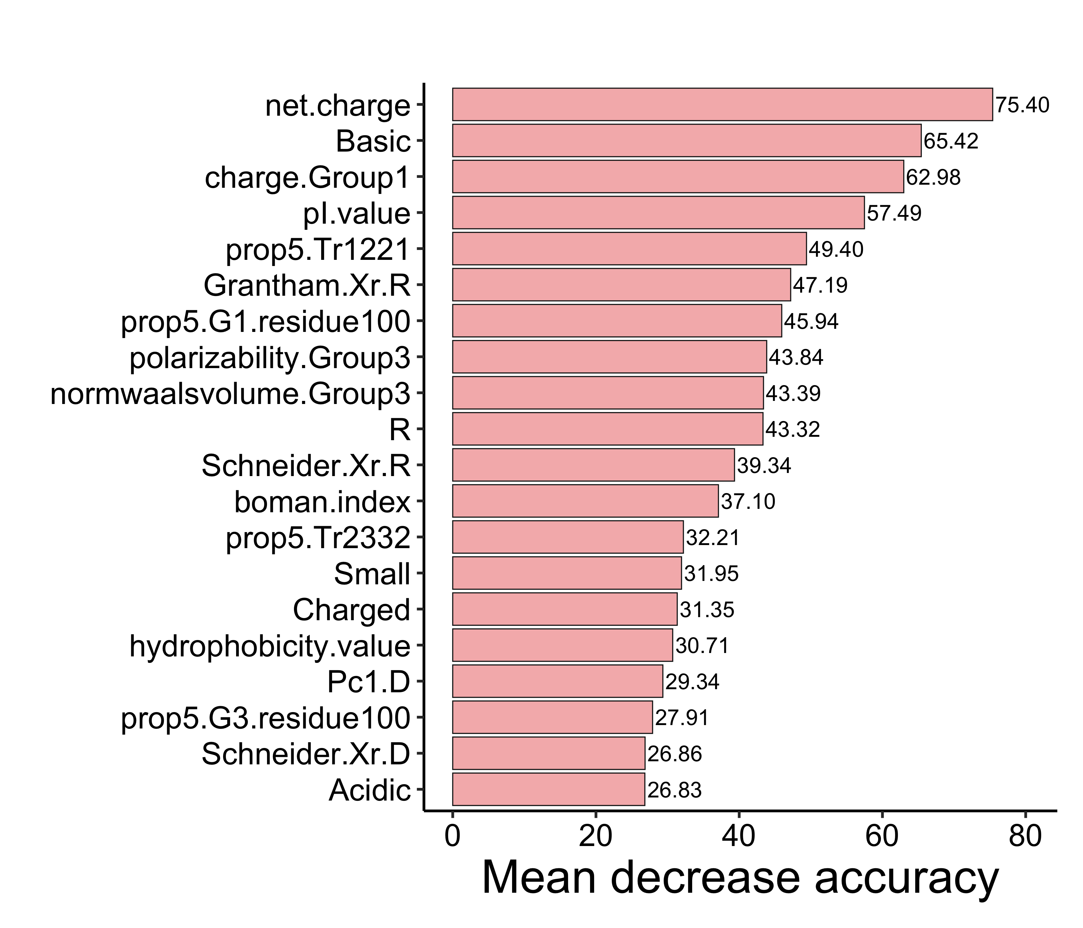
sessionInfo()## R version 4.2.2 (2022-10-31)
## Platform: x86_64-apple-darwin17.0 (64-bit)
## Running under: macOS Big Sur ... 10.16
##
## Matrix products: default
## BLAS: /Library/Frameworks/R.framework/Versions/4.2/Resources/lib/libRblas.0.dylib
## LAPACK: /Library/Frameworks/R.framework/Versions/4.2/Resources/lib/libRlapack.dylib
##
## locale:
## [1] en_US.UTF-8/en_US.UTF-8/en_US.UTF-8/C/en_US.UTF-8/en_US.UTF-8
##
## attached base packages:
## [1] stats graphics grDevices utils datasets methods base
##
## other attached packages:
## [1] ggplot2_3.3.6 randomForest_4.7-1.1 plyr_1.8.7
## [4] protr_1.6-2 stringr_1.4.1 Peptides_2.4.4
## [7] seqinr_4.2-16
##
## loaded via a namespace (and not attached):
## [1] styler_1.8.0 tidyselect_1.1.2 xfun_0.32 bslib_0.4.0
## [5] purrr_0.3.4 colorspace_2.0-3 vctrs_0.4.1 generics_0.1.3
## [9] htmltools_0.5.3 yaml_2.3.5 utf8_1.2.2 rlang_1.0.4
## [13] R.oo_1.25.0 jquerylib_0.1.4 pillar_1.8.1 glue_1.6.2
## [17] withr_2.5.0 DBI_1.1.3 R.utils_2.12.0 R.cache_0.16.0
## [21] lifecycle_1.0.1 munsell_0.5.0 gtable_0.3.0 R.methodsS3_1.8.2
## [25] codetools_0.2-18 evaluate_0.16 knitr_1.40 fastmap_1.1.0
## [29] fansi_1.0.3 highr_0.9 Rcpp_1.0.9 scales_1.2.1
## [33] cachem_1.0.6 jsonlite_1.8.0 digest_0.6.29 stringi_1.7.8
## [37] bookdown_0.28 dplyr_1.0.9 grid_4.2.2 ade4_1.7-19
## [41] cli_3.3.0 tools_4.2.2 magrittr_2.0.3 sass_0.4.2
## [45] tibble_3.1.8 pkgconfig_2.0.3 MASS_7.3-58.1 assertthat_0.2.1
## [49] rmarkdown_2.16 rstudioapi_0.14 R6_2.5.1 compiler_4.2.2