Section 4 Model validation and interpretation
library(h2o)
library(ggplot2)
library(ggpubr)
library(ggbeeswarm)
library(reticulate)
use_condaenv("/Users/renee/Library/r-miniconda/envs/peptide_engineering/bin/python")
library(reshape2)
library(scales)
library(ggforce)
library(cowplot)
library(plotly)
library(ggrepel)
import h2o
import pandas as pd
import numpy as np
import shap
import matplotlib.pyplot as plt
import session_info4.1 Model validation
4.1.1 Melaning binding
# ================
# predicted values
# ================
mb_pred_ <- matrix(
  c(
    -0.0202, 1.3650, 2.1745, 2.3456, 2.5907, 2.6903, 2.9842, 3.1325, 3.5015, 3.6640, 3.7181, 4.0701,
    0.3223, 1.5153, 2.1196, 2.4047, 2.5032, 2.8177, 3.0653, 3.1491, 3.5578, 3.6465, 3.5599, 3.9509,
    0.6579, 2.1797, 1.9685, 2.3709, 2.6702, 3.0694, 2.9323, 3.3150, 3.4798, 3.5661, 3.6981, 3.9730,
    -0.0589, 1.3490, 2.4402, 2.1269, 2.5097, 2.6128, 2.9359, 3.3530, 3.8094, 3.5260, 3.7525, 3.8405,
    0.6532, 1.3684, 2.6170, 2.5270, 2.5228, 2.9967, 3.1125, 3.2106, 3.5952, 3.7345, 3.7353, 3.8400,
    0.2941, 1.1896, 2.1987, 2.7585, 3.1348, 2.9791, 3.2625, 3.0559, 3.5153, 3.6829, 3.9875, 4.0330,
    0.0156, 1.1113, 1.9551, 2.3677, 2.4250, 4.0111, 3.4891, 3.6521, 3.6634, 3.2731, 3.4504, 3.7587,
    0.0209, 1.9146, 2.2865, 2.5308, 2.7193, 3.0322, 3.1020, 3.3582, 3.2993, 3.8534, 4.9542, 3.5464
  ),
  nrow = 8, byrow = TRUE
)

new_mb_pred_ <- c(
  3.9318, 3.9366, 3.5531, 3.4385, 3.8434, 3.3893, 4.4159, 4.7549, 4.0004, 3.2785,
  4.5784, 4.6026, 3.6229, 3.8261, 3.6111, 5.0536, 4.8169, 5.9021, 4.0992, 4.3451,
  5.9626, 4.2730, 4.4115, 4.8889, 4.3264, 4.4830, 4.2847, 4.6585, 4.4568, 4.8513,
  4.1523
)

mb_pred <- c(as.vector(mb_pred_), new_mb_pred_)
for (i in 1:127) {
  if (mb_pred[i] < 0) mb_pred[i] <- NA
}
# Re-scale to 0-100
load(file = "./rdata/var_reduct_mb_train_test_splits.RData")
mb_pred <- rescale(mb_pred, to = c(0, 100), from = range(mb_data$log_intensity))
mb_pred[mb_pred > 100] <- 100

# ===================
# Experimental values
# ===================
replicate_1_1 <- matrix(
  c(
    0.9775, 50.1718, 39.9822, 66.0486, 46.0249, 40.8353, 58.6552, 72.8258, 55.1955, 59.8874, 78.4182, 77.8258,
    -3.6197, 25.3377, 56.6884, 58.1339, -0.8945, 26.5936, 64.4609, 63.2050, 68.3472, 71.3566, 80.4325, 70.3140,
    -34.7571, 26.0249, 52.3519, 70.4562, 63.1813, 69.1291, 73.1339, 65.6220, 73.9396, 76.5699, 75.1955, 76.0249,
    -1.3922, 35.4325, 4.0344, 16.4514, 28.4656, 38.9870, 71.5699, 66.8306, 71.0723, 45.0059, 83.4182, 75.9301,
    -6.0604, 19.9111, 20.2666, 39.2476, 36.3329, 70.1955, 73.9633, 72.4467, 75.5746, 59.9348, 55.4799, 75.8590,
    1.9727, 28.0628, -29.7097, 35.4562, 58.8211, 49.7927, 61.7121, 77.8732, 77.2097, 77.2571, 54.8874, 76.0249,
    -23.3353, 33.2998, 45.9064, 36.1671, 36.4751, 74.5557, 70.6220, 48.2998, 69.6742, 76.9727, 65.1244, 75.9064,
    2.2571, 27.1860, -1.6055, 42.3519, 48.7500, 47.8969, 62.2334, 70.6220, 79.7927, 75.9538, 77.4467, 81.0960
  ),
  nrow = 8, byrow = TRUE
)

replicate_1_2 <- matrix(
  c(
    -7.7192, 54.0818, 45.1007, 62.8495, 50.1481, 37.6126, 59.5083, 71.7121, 57.7073, 59.4135, 77.0201, 82.3756,
    21.4277, 10.8353, 54.6268, 65.7168, 15.6220, 35.1007, 64.8637, 67.8258, 66.5225, 72.7073, 83.1576, 72.7784,
    -53.7855, 2.6600, 42.8732, 32.9443, 48.1576, 71.0960, 73.4656, 66.9964, 72.1386, 78.6789, 78.7500, 77.1386,
    34.9822, 37.1623, 25.8590, 34.7453, 36.9964, 54.2239, 72.8969, 67.5415, 73.5604, 52.8021, 88.1339, 80.0296,
    1.1434, 30.6694, 32.8969, 45.5983, 48.6552, 70.5036, 74.7927, 76.0249, 75.5983, 62.6600, 61.3803, 81.4277,
    27.4467, 30.3614, 24.8164, 25.8116, 63.9633, 49.7927, 60.6457, 79.8637, 77.3282, 79.8164, 55.0770, 77.1386,
    7.9206, 44.0107, 57.2571, 50.1955, 45.6220, 76.2618, 71.7358, 51.6410, 72.9680, 76.6410, 64.1291, 76.5225,
    -3.7618, 32.5178, 28.9159, 47.3756, 50.5983, 49.4609, 62.7547, 71.7358, 83.3709, 81.7832, 83.3235, 82.9917
  ),
  nrow = 8, byrow = TRUE
)

replicate_2_1 <- matrix(
  c(
    -21.6291, 12.7784, 51.7595, 30.0770, 33.6078, 28.2524, 47.4467, 51.8780, 45.4088, 64.9585, 64.9585, 69.3187,
    24.2476, 7.0675, 56.8780, 71.7595, 25.8116, 40.1481, 69.2476, 71.3803, 74.9585, 73.1813, 81.8069, 74.8400,
    44.5557, 31.2618, 43.6552, 39.0818, 48.3235, 67.8495, 76.2855, 64.5557, 74.5083, 76.0723, 75.4799, 75.5746,
    17.3045, 45.8590, -7.5533, 34.7690, 28.3945, 41.9491, 73.3709, 69.8874, 70.1244, 62.9206, 71.8306, 78.6552,
    17.0675, 34.8874, 19.2002, 35.7168, 43.5130, 2.1386, 70.8353, 50.4325, 73.8922, 68.7974, 76.4277, 77.3756,
    51.4751, 2.5652, 13.2998, 25.7405, 58.7500, 50.5036, 64.6979, 76.6410, 67.4467, 80.3614, 63.3945, 75.5746,
    -41.2500, 44.1528, 51.4040, 35.3377, 57.3993, 78.3945, 72.7784, 56.4751, 75.5746, 74.5320, 68.5604, 75.0533,
    15.5036, 31.6173, 11.4040, 49.9111, 49.6505, 48.0865, 61.4040, 72.7784, 79.9822, 77.9443, 71.5699, 79.8164
  ),
  nrow = 8, byrow = TRUE
)

replicate_2_2 <- matrix(
  c(
    13.5367, 25.8827, 48.0628, 76.2855, 58.0628, 54.2713, 69.7927, 78.9633, 55.6457, 78.2287, 80.5983, 83.6789,
    51.5699, 6.1671, 50.8116, 73.3472, 28.4419, 26.0960, 73.4893, 76.5699, 74.5320, 78.7263, 85.4799, 80.1718,
    41.7595, 48.1339, 39.0818, 43.8211, 47.9917, 65.2429, 79.1765, 73.6078, 78.5604, 82.7547, 81.2855, 82.6126,
    38.0154, 30.6931, 42.3045, 41.2145, 30.7642, 57.1386, 75.6220, 70.5746, 72.1386, 66.0960, 78.2287, 80.9775,
    19.6742, 25.1481, 36.0012, 28.8685, 33.3472, 70.0533, 73.1102, 55.5509, 73.3945, 74.7216, 80.4325, 80.8827,
    46.7832, 28.2050, 30.6220, 30.2903, 60.5036, 34.1291, 66.9964, 77.6363, 76.3803, 85.6694, 68.1102, 82.6126,
    6.4040, 24.1528, 64.3661, 47.6126, 63.5604, 81.3566, 79.8164, 61.2382, 78.0628, 78.5604, 70.7405, 76.9017,
    25.3140, 42.5889, 40.6694, 50.2192, 53.0154, 47.0912, 66.6173, 79.8164, 83.3709, 82.6363, 77.1623, 84.3898
  ),
  nrow = 8, byrow = TRUE
)

replicate_1_1 <- as.vector(replicate_1_1)
replicate_1_2 <- as.vector(replicate_1_2)
replicate_2_1 <- as.vector(replicate_2_1)
replicate_2_2 <- as.vector(replicate_2_2)

mb_true_ <- c()
for (i in 1:96) {
  res_ <- mean(c(
    mean(c(replicate_1_1[i], replicate_1_2[i])),
    mean(c(replicate_2_1[i], replicate_2_2[i]))
  ))
  if (res_ >= 0) {
    mb_true_ <- c(mb_true_, res_)
  } else {
    mb_true_ <- c(mb_true_, NA)
  }
}

new_replicate_1 <- c(
  79.9064, 80.2179, 75.9474, 79.1975, 71.6238, 53.5235, 83.5678, 81.2452, 74.2512, 68.4291,
  90.2855, 89.2512, 92.8356, 80.2853, 62.0912, 89.2853, 70.1267, 90.2891, 63.2853, 70.6812,
  89.2582, 85.2567, 78.3682, 90.5732, 82.5253, 84.2912, 82.5923, 90.8613, 73.2862, 90.4823,
  59.2715
)

new_replicate_2 <- c(
  77.6257, 82.2692, 71.8684, 79.1338, 67.7994, 52.3258, 88.2912, 79.6823, 78.5257, 62.5212,
  81.2842, 83.5812, 90.2512, 73.4821, 63.6843, 88.2965, 72.0582, 93.1925, 62.9142, 78.0396,
  86.9323, 82.5323, 72.6429, 83.6736, 89.5191, 86.8432, 81.5171, 92.1856, 92.6736, 93.9124,
  95.3929
)

new_replicate_3 <- c(
  79.7602, 83.5192, 74.6645, 80.8854, 67.3918, 49.5821, 93.1263, 84.2590, 76.9253, 60.4827,
  93.4825, 85.9901, 88.5705, 79.0125, 60.1825, 90.5812, 71.2281, 89.9251, 64.2681, 72.5712,
  83.9235, 84.2719, 71.1281, 95.2182, 90.0191, 89.1812, 82.7195, 89.9501, 83.8581, 85.3725,
  93.2801
)

new_mb_true_ <- c()
for (i in 1:31) {
  res_ <- mean(c(new_replicate_1[i], new_replicate_2[i], new_replicate_3[i]))
  if (res_ >= 0) {
    new_mb_true_ <- c(new_mb_true_, res_)
  } else {
    new_mb_true_ <- c(new_mb_true_, NA)
  }
}

mb_true <- c(mb_true_, new_mb_true_)
mb_df <- data.frame(mb_pred = mb_pred, mb_true = mb_true)
mb_df <- mb_df[complete.cases(mb_df), ]
p1 <- ggscatter(mb_df,
x = "mb_pred", y = "mb_true",
alpha = 0.8, size = 2.5, stroke = 0.2, color = "black", fill = "grey70", shape = 21,
add = "reg.line", conf.int = TRUE, conf.int.level = 0.95, cor.coef = TRUE,
add.params = list(color = "grey25", fill = "grey70"),
cor.coeff.args = list(
method = "pearson", label.x = 2, label.y = 95, label.sep = "\n",
size = 4.5
)
) +
theme_bw() +
theme(
panel.grid.major = element_blank(),
panel.grid.minor = element_blank(),
strip.background = element_blank(),
panel.border = element_blank(),
axis.line = element_line(color = "black"),
axis.title.x = element_text(colour = "black", size = 15),
axis.title.y = element_text(colour = "black", size = 15),
axis.text.x = element_text(colour = "black", size = 12),
axis.text.y = element_text(colour = "black", size = 12)
) +
xlab("Predicted peptide bound\nto b-mNPs (%)") +
ylab("Measured peptide bound\nto mNPs (%)") +
xlim(-5, 105) +
ylim(-5, 105)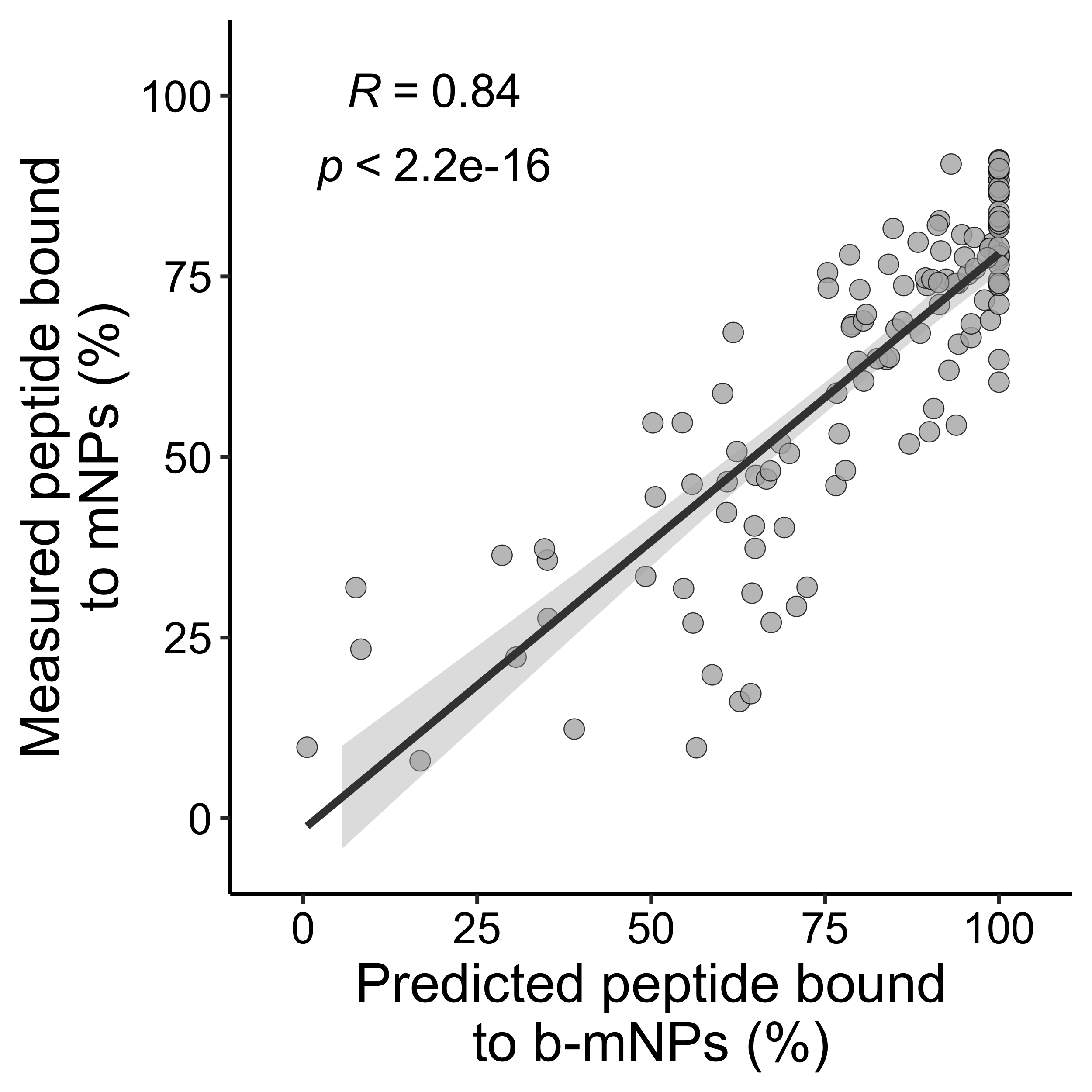
4.1.2 Melanin binding and cell-penetration
# ================
# predicted values
# ================
cpp_pred_ <- matrix(
  c(
    "Non-CPP", "Non-CPP", "CPP", "CPP", "CPP", "CPP", "CPP", "CPP", "CPP", "CPP", "CPP", "CPP",
    "Non-CPP", "CPP", "CPP", "CPP", "CPP", "CPP", "CPP", "CPP", "CPP", "CPP", "CPP", "CPP",
    "Non-CPP", "CPP", "CPP", "CPP", "CPP", "CPP", "CPP", "CPP", "CPP", "CPP", "CPP", "CPP",
    "CPP", "CPP", "CPP", "CPP", "CPP", "CPP", "CPP", "CPP", "CPP", "CPP", "CPP", "CPP",
    "CPP", "CPP", "CPP", "CPP", "CPP", "CPP", "CPP", "CPP", "CPP", "CPP", "CPP", "CPP",
    "Non-CPP", "Non-CPP", "CPP", "CPP", "CPP", "CPP", "CPP", "CPP", "CPP", "CPP", "CPP", "CPP",
    "Non-CPP", "Non-CPP", "Non-CPP", "CPP", "CPP", "CPP", "CPP", "CPP", "CPP", "CPP", "CPP", "CPP",
    "Non-CPP", "Non-CPP", "Non-CPP", "Non-CPP", "Non-CPP", "CPP", "CPP", "CPP", "CPP", "CPP", "CPP", "CPP"
  ),
  nrow = 8, byrow = TRUE
)

new_cpp_pred_ <- c(
  "CPP", "CPP", "CPP", "CPP", "CPP", "CPP", "CPP", "CPP", "CPP", "CPP",
  "CPP", "CPP", "CPP", "CPP", "CPP", "CPP", "CPP", "CPP", "CPP", "CPP",
  "CPP", "CPP", "CPP", "CPP", "CPP", "CPP", "CPP", "CPP", "CPP", "CPP",
  "CPP"
)

cpp_pred <- c(as.vector(cpp_pred_), new_cpp_pred_)

# ===================
# Experimental values
# ===================
non_induced_replicate_1 <- matrix(
  c(
    31.3344, 24.1344, 25.3344, 45.4944, 16.0944, 146.6544, 20.2944, 18.9744, 15.3744, 12.0144, 19.8144, 15.3744,
    20.8944, 20.1744, 17.2944, 63.1344, 15.6144, 15.6144, 32.4144, 16.5744, 17.7744, 12.1344, 14.7744, 55.9344,
    19.4544, 21.3744, 29.1744, 25.9344, 89.5344, 14.8944, 19.9344, 11.4144, 29.5344, 13.5744, 13.3344, 33.9744,
    13.2144, 8.1744, 29.7744, -24.8256, 14.2944, 18.4944, 15.7344, 14.6544, 14.1744, 10.9344, 9.1344, 55.6944,
    13.9344, 12.8544, 36.7344, 20.8944, 15.2544, 17.5344, 13.3344, 17.4144, 20.7744, 10.9344, 15.8544, 19.4544,
    10.4544, 20.2944, 25.9344, 19.9344, 18.8544, 15.8544, 15.7344, 20.2944, 13.4544, 7.5744, 11.7744, 33.9744,
    17.7744, 24.8544, 23.6544, 19.5744, 19.9344, 77.5344, 24.0144, 24.8544, 24.4944, 29.5344, 31.5744, 53.8944,
    9.7344, 10.5744, 25.3344, 15.7344, 27.9744, 27.4944, 19.6944, 19.4544, 27.4944, 24.4944, 24.6144, 26.2944
  ),
  nrow = 8, byrow = TRUE
)

non_induced_replicate_2 <- matrix(
  c(
    30.3744, 28.4544, 26.1744, 30.0144, 25.6944, 131.5344, 31.8144, 21.9744, 30.4944, 20.2944, 17.7744, 26.7744,
    27.4944, 20.6544, 21.3744, 44.2944, 23.6544, 28.5744, 26.5344, 22.0944, 26.7744, 17.5344, 18.9744, 63.0144,
    25.6944, 22.8144, 27.6144, 26.7744, 88.9344, 30.8544, 24.1344, 10.9344, 19.9344, 19.5744, 21.4944, 25.2144,
    12.9744, 15.0144, 17.7744, 14.8944, 13.5744, 24.4944, 27.6144, 13.9344, 23.1744, 17.7744, 15.7344, 45.6144,
    16.0944, 23.1744, 17.7744, 15.7344, 20.6544, 27.6144, 34.0944, 24.6144, 22.8144, 14.4144, 26.7744, 25.6944,
    12.0144, 31.8144, 16.4544, 21.6144, 30.2544, 18.7344, 24.9744, 29.7744, 15.1344, 15.1344, 27.8544, 25.2144,
    23.2944, 28.2144, 30.6144, 22.0944, 19.9344, 63.0144, 22.8144, 22.2144, 21.6144, 19.9344, 23.0544, 30.9744,
    14.0544, 23.7744, 20.6544, 11.0544, 23.8944, 31.4544, 20.6544, 15.4944, 31.4544, 26.0544, 33.0144, 37.0944
  ),
  nrow = 8, byrow = TRUE
)

non_induced_replicate_3 <- matrix(
  c(
    27.3744, 16.3344, 17.5344, 33.7344, 13.8144, 110.8944, 33.4944, 37.2144, 34.8144, 20.8944, 39.4944, 36.1344,
    15.9744, 13.4544, 18.6144, 28.2144, 13.0944, 12.8544, 46.3344, 27.6144, 64.6944, 3.4944, 25.5744, 40.8144,
    13.8144, 13.5744, 35.7744, 16.4544, 54.4944, 14.2944, 30.7344, 23.6544, 41.0544, 8.5344, 23.1744, 52.2144,
    32.5344, 19.4544, 27.2544, 27.1344, 20.5344, 27.3744, 30.6144, 25.6944, 27.1344, 28.3344, 29.4144, 27.3744,
    30.0144, 19.5744, 31.3344, 31.9344, 25.6944, 26.7744, 36.4944, 25.8144, 35.2944, 7.8144, 45.1344, 21.7344,
    19.4544, 33.4944, 22.8144, 19.8144, 21.9744, 22.8144, 24.8544, 29.4144, 31.3344, 33.3744, 42.9744, 52.2144,
    12.4944, 15.3744, 27.3744, 10.4544, 7.9344, 64.3344, 36.0144, 68.7744, 27.6144, 41.0544, 47.5344, 70.2144,
    20.4144, 10.8144, 28.0944, 20.5344, 29.0544, 37.2144, 27.9744, 14.1744, 37.2144, 29.4144, 23.1744, 25.5744
  ),
  nrow = 8, byrow = TRUE
)

non_induced_true_ <- c()
for (i in 1:96) {
  res_ <- mean(c(non_induced_replicate_1[i], non_induced_replicate_2[i], non_induced_replicate_3[i]))
  non_induced_true_ <- c(non_induced_true_, res_)
}

induced_replicate_1 <- matrix(
  c(
    171.4944, 32.1744, 23.6544, 24.7344, 47.1744, 404.5344, 224.2944, 71.8944, 442.4544, 394.5744, 294.8544, 464.8944,
    39.4944, 24.2544, 59.4144, 55.6944, 31.9344, 182.2944, 195.2544, 434.1744, 486.8544, 406.8144, 25.4544, 524.5344,
    28.8144, 76.2144, 160.6944, 32.6544, 424.8144, 60.4944, 474.1344, 281.2944, 240.2544, 226.8144, 386.1744, 235.2144,
    20.7744, 28.9344, 43.6944, 34.2144, 20.6544, 45.9744, 297.0144, 30.9744, 540.3744, 235.4544, 618.3744, 395.7744,
    24.7344, 13.9344, 30.2544, 23.5344, 14.8944, 17.1744, 40.5744, 132.4944, 410.4144, 53.2944, 352.8144, 427.2144,
    13.3344, 224.2944, 28.2144, 48.0144, 62.5344, 25.6944, 352.6944, 245.6544, 80.8944, 313.5744, 414.6144, 235.2144,
    20.8944, 29.8944, 36.9744, 19.6944, 12.7344, 422.1744, 341.8944, 120.2544, 333.6144, 281.2944, 534.7344, 356.2944,
    15.7344, 66.4944, 33.3744, 21.0144, 73.5744, 17.8944, 108.9744, 116.1744, 618.3744, 538.0944, 554.0544, 502.4544
  ),
  nrow = 8, byrow = TRUE
)

induced_replicate_2 <- matrix(
  c(
    39.1344, 30.1344, 34.5744, 367.2144, 36.7344, 185.4144, 192.9744, 434.2944, 376.2144, 305.4144, 192.9744, 420.6144,
    41.4144, 19.4544, 101.6544, 370.0944, 43.9344, 231.1344, 110.1744, 476.8944, 395.6544, 315.6144, 75.9744, 435.2544,
    26.8944, 60.6144, 29.8944, 200.1744, 460.5744, 265.9344, 541.6944, 310.2144, 282.6144, 404.4144, 168.9744, 196.2144,
    12.6144, 137.7744, 16.0944, 16.2144, 47.8944, 24.7344, 274.4544, 62.0544, 247.9344, 209.2944, 393.4944, 423.3744,
    22.2144, 21.3744, 11.1744, 9.1344, 128.4144, 19.6944, 58.9344, 233.1744, 437.4144, 58.6944, 361.0944, 458.8944,
    16.8144, 33.3744, 12.3744, 24.3744, 134.1744, 25.9344, 364.4544, 207.8544, 91.2144, 383.6544, 434.0544, 196.2144,
    11.8944, 21.7344, 17.4144, 16.8144, 19.9344, 525.4944, 422.4144, 519.9744, 379.5744, 282.6144, 616.9344, 450.0144,
    19.2144, 42.7344, 19.4544, 25.9344, 54.7344, 42.9744, 73.2144, 135.4944, 524.0544, 471.7344, 528.4944, 511.0944
  ),
  nrow = 8, byrow = TRUE
)

induced_replicate_3 <- matrix(
  c(
    30.3744, 20.2944, 233.8944, 83.8944, 24.2544, 25.3344, 136.2144, 374.8944, 334.5744, 399.6144, 383.6544, 544.6944,
    18.9744, 21.1344, 20.0544, 401.7744, 22.6944, 62.7744, 51.4944, 430.6944, 303.7344, 466.6944, 329.6544, 567.7344,
    21.8544, 75.3744, 51.9744, 150.3744, 411.4944, 122.0544, 458.2944, 127.8144, 38.4144, 269.8944, 51.9744, 366.9744,
    12.1344, 6.6144, 8.8944, 16.8144, 13.3344, 24.4944, 276.9744, 77.4144, 163.6944, 297.8544, 423.9744, 492.8544,
    13.9344, 1.9344, 10.4544, 10.5744, 19.0944, 17.6544, 33.0144, 86.7744, 43.2144, 316.0944, 382.8144, 351.9744,
    1.4544, 136.2144, 9.9744, 13.4544, 101.5344, 18.1344, 403.9344, 183.0144, 389.7744, 70.4544, 444.1344, 149.2944,
    7.5744, 15.3744, 141.7344, 15.0144, 12.1344, 423.4944, 422.7744, 94.8144, 269.8944, 289.2144, 473.7744, 364.5744,
    0.8544, 25.5744, 14.4144, 8.4144, 37.3344, 37.2144, 250.5744, 159.3744, 608.5344, 466.2144, 524.4144, 510.4944
  ),
  nrow = 8, byrow = TRUE
)

induced_true_ <- c()
for (i in 1:96) {
  res_ <- mean(c(induced_replicate_1[i], induced_replicate_2[i], induced_replicate_3[i]))
  induced_true_ <- c(induced_true_, res_)
}

new_non_induced_replicate_1 <- c(
  94.6865, 84.2145, 58.6890, 69.1610, 35.1270, 12.4261, 19.8169, 12.4261, 12.4368, 19.8169,
  12.4261, 19.8169, 12.4368, 10.1149, 8.6644,  38.8384, 12.0117, 23.1802, 9.9236,  10.7153,
  55.7665, 14.1476, 24.8167, 11.4644, 21.2568, 41.3144, 11.8948, 17.2878, 21.1505, 12.9894,
  20.8902
)

new_non_induced_replicate_2 <- c(
  88.1415, 77.0150, 52.1440, 43.6355, 35.1270, 11.6132, 28.8335, 11.6132, 13.2019, 28.8335,
  11.6132, 28.8335, 13.2019, 11.6717, 10.0671, 30.3106, 13.4888, 34.5612, 12.9309, 12.6759,
  42.8393, 17.0753, 38.7481, 11.7673, 24.1153, 35.5229, 13.7651, 22.8933, 25.4702, 14.9234,
  29.0832
)

new_non_induced_replicate_3 <- c(
  64.5795, 63.2705, 48.2170, 52.1440, 27.9275, 15.0881, 40.0817, 15.0881, 13.9936, 40.0817,
  15.0881, 40.0817, 13.9936, 8.5847, 13.4835, 64.9266, 13.2444, 56.1065, 10.6090, 13.8660,
  69.1400, 21.0974, 67.0891, 10.8056, 25.8900, 55.3361, 16.4695, 24.6201, 42.7755, 14.1317,
  49.6828
)

new_non_induced_true_ <- c()
for (i in 1:31) {
  res_ <- mean(c(new_non_induced_replicate_1[i], new_non_induced_replicate_2[i], new_non_induced_replicate_3[i]))
  new_non_induced_true_ <- c(new_non_induced_true_, res_)
}

new_induced_replicate_1 <- c(
  775.3412, 608.3964, 376.3855, 403.2684, 450.2610, 104.3842, 610.9376, 104.3842, 206.0770, 610.9376,
  104.3842, 610.9376, 206.0770, 61.42746, 63.9640, 725.5767, 182.7868, 436.4094, 89.5931, 105.8666,
  643.6163, 295.6471, 536.2245, 141.8066, 415.8205, 549.5332, 258.9823, 532.0408, 386.370, 313.6335,
  596.1610
)

new_induced_replicate_2 <- c(
  720.8794, 670.3267, 402.6897, 361.0000, 423.5832, 95.4568, 353.5596, 95.4568, 173.0359, 353.5596,
  95.4568, 353.5596, 173.0359, 70.6842, 58.2979, 560.2724, 235.8898, 367.2965, 83.7953, 102.8688,
  552.6956, 249.6267, 461.8738, 114.8928, 335.8037, 455.3512, 205.2205, 327.7658, 417.4017, 186.3116,
  851.0120
)

new_induced_replicate_3 <- c(
  783.3711, 690.3612, 393.6819, 493.6712, 480.9125, 86.2659, 417.0393, 86.2659, 159.3978, 417.0393,
  86.2659, 417.0393, 159.3978, 60.1427, 53.6201, 512.8355, 120.0977, 394.4739, 100.9911, 112.4550,
  577.1388, 243.4006, 552.0697, 118.0552, 376.5862, 513.8896, 224.0635, 387.4242, 380.8028, 221.7246,
  766.4130
)

new_induced_true_ <- c()
for (i in 1:31) {
  res_ <- mean(c(new_induced_replicate_1[i], new_induced_replicate_2[i], new_induced_replicate_3[i]))
  new_induced_true_ <- c(new_induced_true_, res_)
}

cpp_true_non_induced <- c(non_induced_true_, new_non_induced_true_)
cpp_true_induced <- c(induced_true_, new_induced_true_)
mb_cp_df <- data.frame(
mb_true = rep(mb_true, 2),
cpp_true = c(cpp_true_non_induced, cpp_true_induced),
mb_pred = rep(mb_pred, 2),
cpp_pred = factor(rep(cpp_pred, 2), levels = c("Non-CPP", "CPP")),
cell_group = as.factor(c(
rep("Non-induced", length(cpp_true_non_induced)),
rep("Induced", length(cpp_true_induced))
))
)4.1.3 Melanin-induced cells
mb_cp_df$log_cpp_true <- log10(mb_cp_df$cpp_true)
p2_1 <- ggscatter(mb_cp_df[mb_cp_df$cell_group == "Induced", ],
  x = "mb_true", y = "log_cpp_true",
  alpha = 0.7, size = 3, stroke = 0.3, color = "black", fill = "cpp_pred", shape = "cpp_pred",
  add = "reg.line", conf.int = TRUE, conf.int.level = 0.95, cor.coef = TRUE,
  add.params = list(color = "grey25"),
  cor.coeff.args = list(
    method = "pearson", label.x = 2.2, label.y = 2.85, label.sep = "\n",
    size = 5
  )
) +
  facet_grid(. ~ cpp_pred) +
  scale_fill_manual(values = c("#1f77b4", "#d62728")) +
  scale_shape_manual(values = c(24, 21)) +
  scale_y_continuous(
    limits = c(0.63, 3),
    breaks = c(1:3, log10(10^(1:4) / 2)),
    labels = sapply(
      c(10^(1:3), 10^(1:4) / 2),
      function(x) format(x, big.mark = ",", scientific = FALSE)
    )
  ) +
  annotation_logticks(sides = "l") +
  guides(fill = "none", shape = "none") +
  theme_bw() +
  theme(
    panel.grid.major = element_blank(),
    panel.grid.minor = element_blank(),
    axis.text.x = element_text(colour = "black", size = 17),
    axis.text.y = element_text(colour = "black", size = 17),
    strip.text = element_text(colour = "black", size = 20),
    panel.border = element_rect(colour = "black"),
    strip.text.y = element_blank(),
    axis.title = element_text(colour = "black", size = 22)
  ) +
  xlab("Peptide bound to mNPs (%)") +
  ylab("Peptide (pMol / 100K cells)")

set.seed(1)
pos <- position_jitter(width = 0.1, seed = 16)
p2_2 <- ggplot(mb_cp_df[mb_cp_df$cell_group == "Induced", ], aes(x = cpp_pred, y = log_cpp_true)) +
  geom_boxplot(aes(color = cpp_pred), outlier.color = NA, lwd = 1.5, show.legend = FALSE) +
  geom_beeswarm(aes(fill = cpp_pred, shape = cpp_pred),
    color = "black", alpha = 0.7, size = 3,
    stroke = 0.3, cex = 2, priority = "random"
  ) +
  stat_compare_means(
    label = "p.signif", size = 5, method = "wilcox.test", label.x.npc = 0.2,
    label.y = 2.92, hide.ns = TRUE
  ) +
  stat_compare_means(
    label = "p.format", size = 5, method = "wilcox.test", label.x.npc = 0.2,
    label.y = 2.82, hide.ns = TRUE
  ) +
  scale_color_manual(values = c("#cae6fa", "#f5b8b8")) +
  scale_fill_manual(values = c("#1f77b4", "#d62728")) +
  scale_shape_manual(values = c(24, 21)) +
  guides(fill = guide_legend(override.aes = list(shape = c(24, 21))), shape = "none") +
  scale_y_continuous(
    limits = c(0.63, 3),
    breaks = c(1:3, log10(10^(1:4) / 2)),
    labels = c(10^(1:3), 10^(1:4) / 2)
  ) +
  annotation_logticks(sides = "l") +
  theme_bw() +
  theme(
    panel.grid.major = element_blank(),
    panel.grid.minor = element_blank(),
    panel.border = element_rect(colour = "black"),
    strip.text = element_text(colour = "black", size = 20),
    axis.text.x = element_text(colour = "black", size = 18),
    legend.text = element_text(colour = "black", size = 15),
    axis.title.y = element_blank(),
    axis.text.y = element_blank(),
    axis.ticks.y = element_blank(),
    plot.margin = unit(c(1.15, 0.15, 0.53, 0), "cm"),
    legend.position = c(0.5, 1.05),
    legend.direction = "horizontal",
    legend.key = element_rect(fill = NA)
  ) +
  xlab("") +
  labs(fill = "", color = "", shape = "")

p2 <- ggarrange(p2_1, p2_2, widths = c(2.39, 1.02))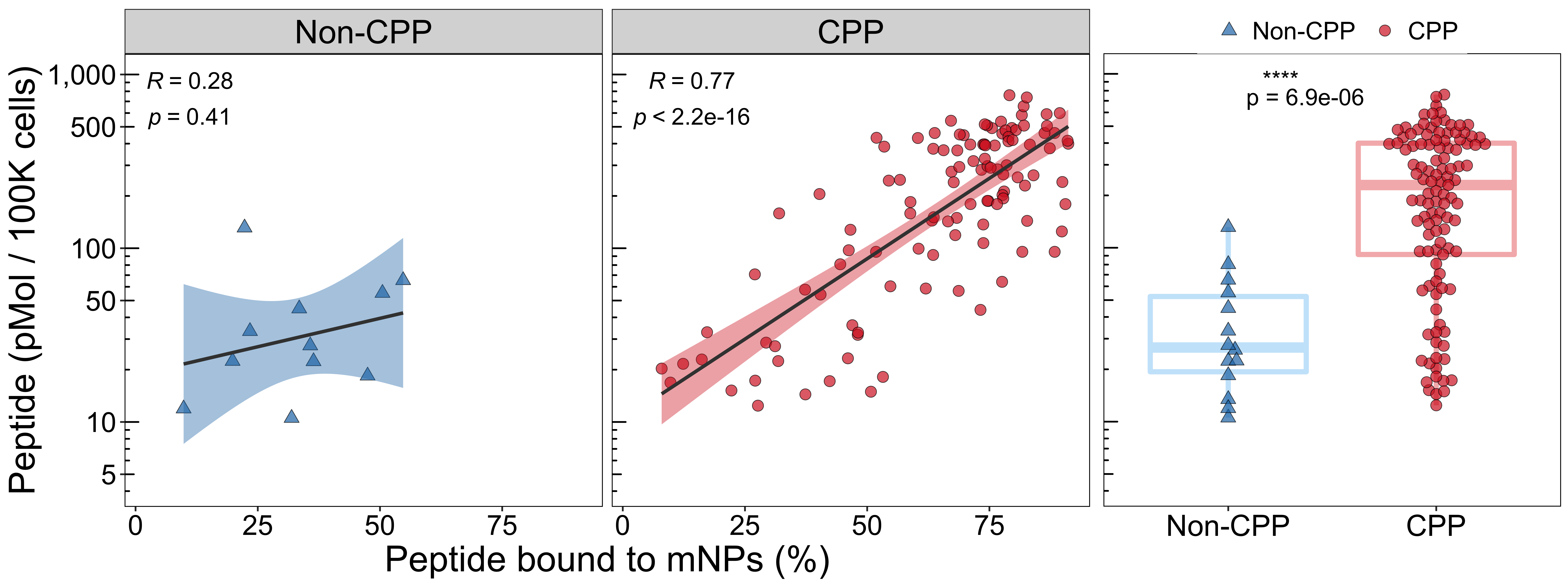
4.1.4 Non-melanin induced cells
p3_1 <- ggscatter(mb_cp_df[mb_cp_df$cell_group == "Non-induced", ],
  x = "mb_true", y = "log_cpp_true",
  alpha = 0.7, size = 3, stroke = 0.3, color = "black", fill = "cpp_pred", shape = "cpp_pred",
  add = "reg.line", conf.int = TRUE, conf.int.level = 0.95, cor.coef = TRUE,
  add.params = list(color = "grey25"),
  cor.coeff.args = list(
    method = "pearson", label.x = 2.2, label.y = 2.85, label.sep = "\n",
    size = 5
  )
) +
  facet_grid(. ~ cpp_pred) +
  scale_fill_manual(values = c("#1f77b4", "#d62728")) +
  scale_shape_manual(values = c(24, 21)) +
  scale_y_continuous(
    limits = c(0.63, 3),
    breaks = c(1:3, log10(10^(1:4) / 2)),
    labels = sapply(
      c(10^(1:3), 10^(1:4) / 2),
      function(x) format(x, big.mark = ",", scientific = FALSE)
    )
  ) +
  annotation_logticks(sides = "l") +
  guides(fill = "none", shape = "none") +
  theme_bw() +
  theme(
    panel.grid.major = element_blank(),
    panel.grid.minor = element_blank(),
    axis.text.x = element_text(colour = "black", size = 17),
    axis.text.y = element_text(colour = "black", size = 17),
    strip.text = element_text(colour = "black", size = 20),
    panel.border = element_rect(colour = "black"),
    strip.text.y = element_blank(),
    axis.title = element_text(colour = "black", size = 22)
  ) +
  xlab("Peptide bound to mNPs (%)") +
  ylab("Peptide (pMol / 100K cells)")

set.seed(1)
pos <- position_jitter(width = 0.1, seed = 16)
p3_2 <- ggplot(mb_cp_df[mb_cp_df$cell_group == "Non-induced", ], aes(x = cpp_pred, y = log_cpp_true)) +
  geom_boxplot(aes(color = cpp_pred), outlier.color = NA, lwd = 1.5, show.legend = FALSE) +
  geom_beeswarm(aes(fill = cpp_pred, shape = cpp_pred),
    color = "black", alpha = 0.7, size = 3,
    stroke = 0.3, cex = 2, priority = "random"
  ) +
  stat_compare_means(
    label = "p.signif", size = 5, method = "wilcox.test", label.x.npc = 0.2,
    label.y = 2.92, hide.ns = TRUE
  ) +
  stat_compare_means(
    label = "p.format", size = 5, method = "wilcox.test", label.x.npc = 0.2,
    label.y = 2.82, hide.ns = TRUE
  ) +
  scale_color_manual(values = c("#cae6fa", "#f5b8b8")) +
  scale_fill_manual(values = c("#1f77b4", "#d62728")) +
  scale_shape_manual(values = c(24, 21)) +
  guides(fill = guide_legend(override.aes = list(shape = c(24, 21))), shape = "none") +
  scale_y_continuous(
    limits = c(0.63, 3),
    breaks = c(1:3, log10(10^(1:4) / 2)),
    labels = c(10^(1:3), 10^(1:4) / 2)
  ) +
  annotation_logticks(sides = "l") +
  theme_bw() +
  theme(
    panel.grid.major = element_blank(),
    panel.grid.minor = element_blank(),
    panel.border = element_rect(colour = "black"),
    strip.text = element_text(colour = "black", size = 20),
    axis.text.x = element_text(colour = "black", size = 18),
    legend.text = element_text(colour = "black", size = 15),
    axis.title.y = element_blank(),
    axis.text.y = element_blank(),
    axis.ticks.y = element_blank(),
    plot.margin = unit(c(1.15, 0.15, 0.53, 0), "cm"),
    legend.position = c(0.5, 1.05),
    legend.direction = "horizontal",
    legend.key = element_rect(fill = NA)
  ) +
  xlab("") +
  labs(fill = "", color = "", shape = "")

p3 <- ggarrange(p3_1, p3_2, widths = c(2.39, 1.02))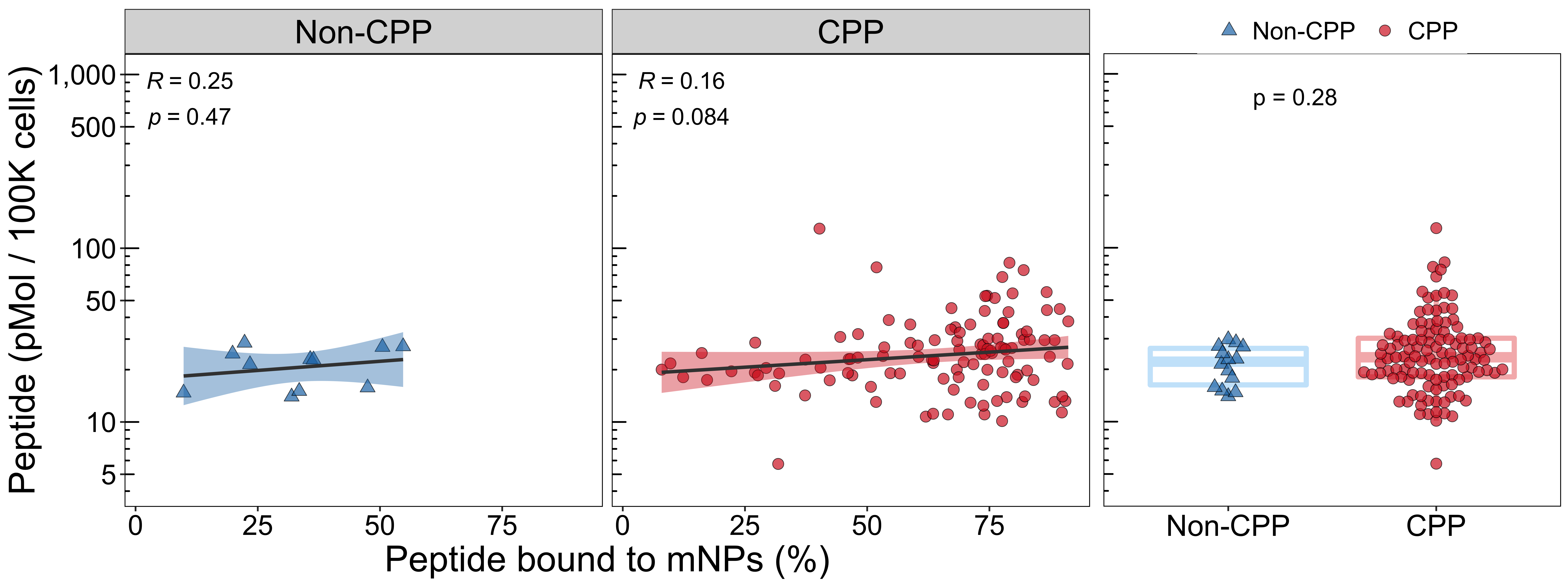
4.2 Overall model interpretation
4.2.1 Melanin binding (regression)
# Save train and test sets in csv format
load(file = "./rdata/var_reduct_mb_train_test_splits.RData")
for (i in 1:10) {
  prefix <- paste0("outer_", i)
  exp_dir <- paste0("/Users/renee/Downloads/melanin_binding/", prefix)
  write.csv(outer_splits[[i]]$train, file = paste0(exp_dir, "/train_set.csv"))
  write.csv(outer_splits[[i]]$test, file = paste0(exp_dir, "/test_set.csv"))
}
exp_dir <- paste0("/Users/renee/Downloads/melanin_binding/whole_data_set")
write.csv(mb_data, file = paste0(exp_dir, "/train_set.csv"))h2o.init(nthreads=-1)
dir_path = '/Users/renee/Downloads/melanin_binding'
model_names = ['superlearner_iter_3', 'superlearner_iter_2', 'superlearner_iter_2', 'superlearner_iter_3',
'superlearner_iter_3', 'superlearner_iter_3', 'superlearner_iter_3', 'superlearner_iter_3',
'superlearner_iter_4', 'superlearner_iter_3']
shap_res = []
for i in range(10):
print('Iter ' + str(i + 1) + ':')
train = pd.read_csv(dir_path + '/outer_' + str(i + 1) + '/train_set.csv', index_col=0)
X_train = train.iloc[:, :-1]
test = pd.read_csv(dir_path + '/outer_' + str(i + 1) + '/test_set.csv', index_col=0)
X_test = test.iloc[:, :-1]
model = h2o.load_model(dir_path + '/outer_' + str(i + 1) + '/' + model_names[i])
def model_predict_(data):
data = pd.DataFrame(data, columns=X_train.columns)
h2o_data = h2o.H2OFrame(data)
res = model.predict(h2o_data)
res = res.as_data_frame()
return(res)
np.random.seed(1)
X_train_ = X_train.iloc[np.random.choice(X_train.shape[0], 100, replace=False), :]
explainer = shap.KernelExplainer(model_predict_, X_train_, link='identity')
shap_values = explainer.shap_values(X_test, nsamples=1000)
shap_res.append(shap_values)
h2o.remove_all()
shap_res = pd.DataFrame(np.vstack(shap_res), columns=X_train.columns)
shap_res.to_csv('./other_data/mb_shap_values_cv_data_sets.csv', index=False)load(file = "./rdata/var_reduct_mb_train_test_splits.RData")
data <- do.call(rbind, lapply(outer_splits, function(x) x$test[-ncol(mb_data)]))
data <- apply(data, 2, function(x) rank(x))
data <- apply(data, 2, function(x) rescale(x, to = c(0, 100)))
shap_values <- as.matrix(read.csv("./other_data/mb_shap_values_cv_data_sets.csv", check.names = FALSE))
shap_values <- as.data.frame(rescale(shap_values, to = c(0, 100), from = range(mb_data$log_intensity)))
var_diff <- apply(shap_values, 2, function(x) max(x) - min(x))
var_diff <- var_diff[order(-var_diff)]
df <- data.frame(
variable = melt(shap_values)$variable,
shap = melt(shap_values)$value,
variable_value = melt(data)$value
)top_vars <- names(var_diff)[1:20]
df <- df[df$variable %in% top_vars, ]
df$variable <- factor(df$variable, levels = rev(top_vars), labels = rev(top_vars))
p1 <- ggplot(df, aes(x = shap, y = variable)) +
geom_hline(yintercept = top_vars, linetype = "dotted", color = "grey80") +
geom_vline(xintercept = 0, color = "grey80", size = 1) +
geom_point(aes(fill = variable_value), color = "grey30", shape = 21, alpha = 0.3, size = 2, position = "auto", stroke = 0.1) +
scale_fill_gradient2(low = "#1f77b4", mid = "white", high = "#d62728", midpoint = 50, breaks = c(0, 100), labels = c("Low", "High")) +
theme_bw() +
theme(
plot.margin = ggplot2::margin(1.5, 8, 1.5, -3),
panel.grid.major = element_blank(),
panel.grid.minor = element_blank(),
strip.background = element_blank(),
panel.border = element_blank(),
axis.line = element_line(color = "black"),
plot.title = element_text(hjust = 0.5, size = 20),
axis.title.x = element_text(hjust = 0.5, colour = "black", size = 20),
axis.title.y = element_text(colour = "black", size = 20),
axis.text.x = element_text(colour = "black", size = 17),
axis.text.y = element_text(colour = "black", size = 16),
legend.title = element_text(size = 20),
legend.text = element_text(colour = "black", size = 16),
legend.title.align = 0.5
) +
guides(
fill = guide_colourbar("Variable\nvalue\n", ticks = FALSE, barheight = 10, barwidth = 0.5),
color = "none"
) +
xlab("SHAP value\n(variable contribution to model prediction)") +
ylab("") +
ggtitle("Melanin binding")
4.2.2 Cell-penetration (classification)
# Save train and test sets in csv format
load(file = "./rdata/var_reduct_cpp_train_test_splits.RData")
for (i in 1:10) {
  prefix <- paste0("outer_", i)
  exp_dir <- paste0("/Users/renee/Downloads/cell_penetration/", prefix)
  write.csv(outer_splits[[i]]$train, file = paste0(exp_dir, "/train_set.csv"))
  write.csv(outer_splits[[i]]$test, file = paste0(exp_dir, "/test_set.csv"))
}
exp_dir <- paste0("/Users/renee/Downloads/cell_penetration/whole_data_set")
write.csv(cpp_data, file = paste0(exp_dir, "/train_set.csv"))h2o.init(nthreads=-1)
dir_path = '/Users/renee/Downloads/cell_penetration'
model_names = ['GBM_model_1669777615732_57632', 'GBM_model_1669777615732_225117', 'GBM_model_1669777615732_387368',
'GBM_model_1669777615732_552677', 'GBM_model_1669777615732_717390', 'GBM_model_1669777538393_67146',
'GBM_model_1669777538393_246060', 'GBM_model_1669777538393_420437', 'GBM_model_1669777538393_602358',
'GBM_model_1669777538393_782798']
shap_res = []
for i in range(10):
print('Iter ' + str(i + 1) + ':')
train = pd.read_csv(dir_path + '/outer_' + str(i + 1) + '/train_set.csv', index_col=0)
X_train = train.iloc[:, :-1]
test = pd.read_csv(dir_path + '/outer_' + str(i + 1) + '/test_set.csv', index_col=0)
X_test = test.iloc[:, :-1]
model = h2o.load_model(dir_path + '/outer_' + str(i + 1) + '/' + model_names[i])
def model_predict_(data):
data = pd.DataFrame(data, columns=X_train.columns)
h2o_data = h2o.H2OFrame(data)
res = model.predict(h2o_data)
res = res.as_data_frame().iloc[:,2]
return(res)
np.random.seed(1)
X_train_ = X_train.iloc[np.random.choice(X_train.shape[0], 100, replace=False), :]
explainer = shap.KernelExplainer(model_predict_, X_train_, link='identity')
shap_values = explainer.shap_values(X_test, nsamples=1000)
shap_res.append(shap_values)
h2o.remove_all()
shap_res = pd.DataFrame(np.vstack(shap_res), columns=X_train.columns)
shap_res.to_csv('./other_data/cpp_shap_values_cv_data_sets.csv', index=False)load(file = "./rdata/var_reduct_cpp_train_test_splits.RData")
data <- do.call(rbind, lapply(outer_splits, function(x) x$test[-ncol(cpp_data)]))
data <- apply(data, 2, function(x) rank(x))
data <- apply(data, 2, function(x) rescale(x, to = c(0, 100)))
shap_values <- read.csv("./other_data/cpp_shap_values_cv_data_sets.csv", check.names = FALSE) * 100
var_diff <- apply(shap_values, 2, function(x) max(x) - min(x))
var_diff <- var_diff[order(-var_diff)]
df <- data.frame(
variable = melt(shap_values)$variable,
shap = melt(shap_values)$value,
variable_value = melt(data)$value
)top_vars <- names(var_diff)[1:11]
df <- df[df$variable %in% top_vars, ]
df$variable <- factor(df$variable, levels = rev(top_vars), labels = rev(top_vars))
p2 <- ggplot(df, aes(x = shap, y = variable)) +
geom_hline(yintercept = top_vars, linetype = "dotted", color = "grey80") +
geom_vline(xintercept = 0, color = "grey80", size = 1) +
geom_point(aes(fill = variable_value), color = "grey30", shape = 21, alpha = 0.5, size = 2, position = "auto", stroke = 0.1) +
scale_fill_gradient2(low = "#1f77b4", mid = "white", high = "#d62728", midpoint = 50, breaks = c(0, 100), labels = c("Low", "High")) +
theme_bw() +
theme(
plot.margin = ggplot2::margin(1.5, 8, 1.5, -3),
panel.grid.major = element_blank(),
panel.grid.minor = element_blank(),
strip.background = element_blank(),
panel.border = element_blank(),
axis.line = element_line(color = "black"),
plot.title = element_text(hjust = 0.5, size = 20),
axis.title.x = element_text(hjust = 0.5, colour = "black", size = 20),
axis.title.y = element_text(colour = "black", size = 20),
axis.text.x = element_text(colour = "black", size = 17),
axis.text.y = element_text(colour = "black", size = 16),
legend.title = element_text(size = 20),
legend.text = element_text(colour = "black", size = 16),
legend.title.align = 0.5
) +
guides(
fill = guide_colourbar("Variable\nvalue\n", ticks = FALSE, barheight = 10, barwidth = 0.5),
color = "none"
) +
xlab("SHAP value\n(variable contribution to model prediction)") +
ylab("") +
ggtitle("Cell-penetration")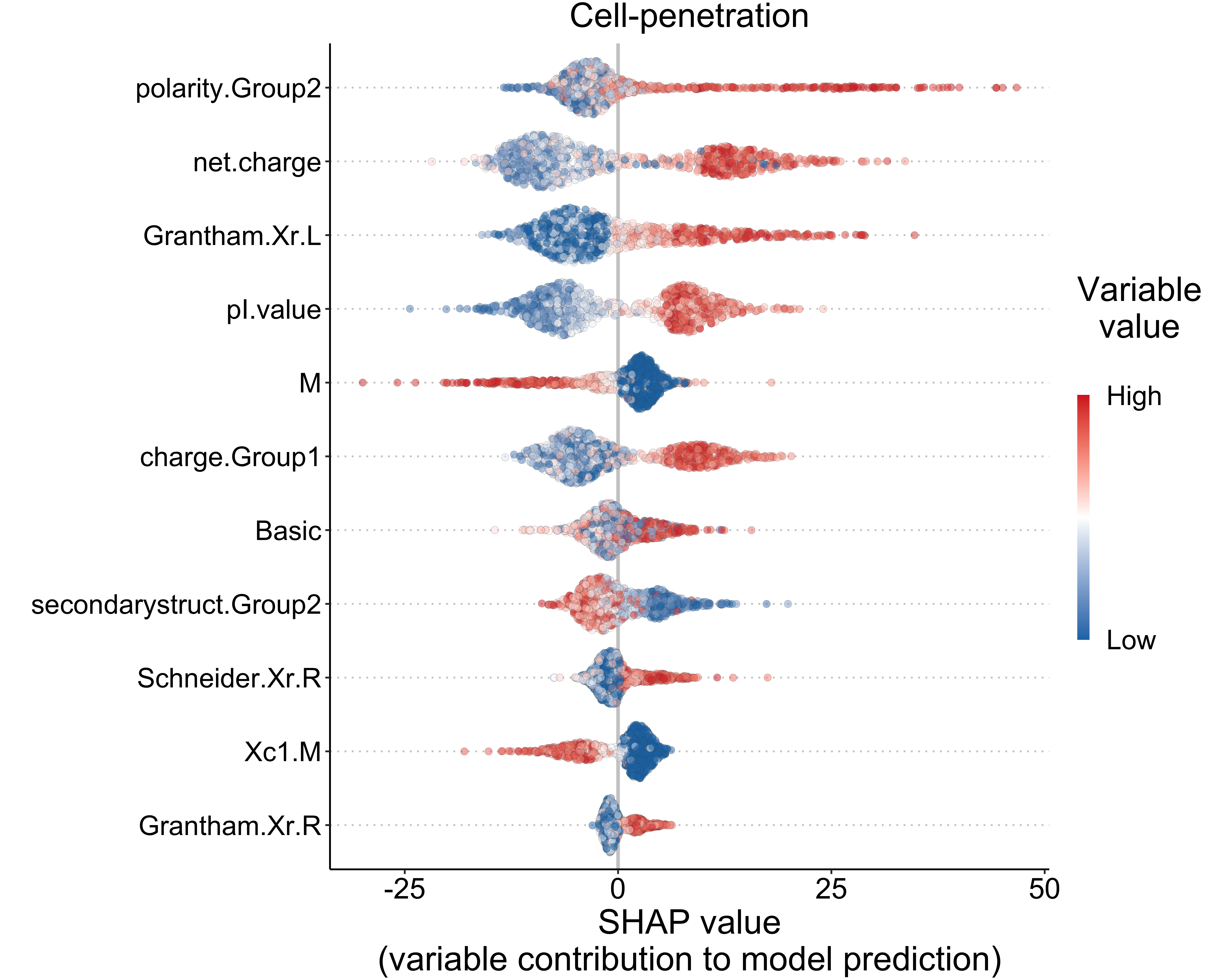
4.2.3 Toxicity (classification)
# Save train and test sets in csv format
load(file = "./rdata/var_reduct_tx_train_test_splits.RData")
for (i in 1:10) {
  prefix <- paste0("outer_", i)
  exp_dir <- paste0("/Users/renee/Downloads/toxicity/", prefix)
  write.csv(outer_splits[[i]]$train, file = paste0(exp_dir, "/train_set.csv"))
  write.csv(outer_splits[[i]]$test, file = paste0(exp_dir, "/test_set.csv"))
}
exp_dir <- paste0("/Users/renee/Downloads/toxicity/whole_data_set")
write.csv(tx_data, file = paste0(exp_dir, "/train_set.csv"))h2o.init(nthreads=-1)
dir_path = '/Users/renee/Downloads/toxicity'
model_names = ['superlearner_iter_4', 'superlearner_iter_3', 'superlearner_iter_3', 'superlearner_iter_3',
'superlearner_iter_3', 'superlearner_iter_3', 'superlearner_iter_3', 'superlearner_iter_4',
'superlearner_iter_3', 'superlearner_iter_4']
shap_res = []
for i in range(10):
print('Iter ' + str(i + 1) + ':')
train = pd.read_csv(dir_path + '/outer_' + str(i + 1) + '/train_set.csv', index_col=0)
X_train = train.iloc[:, :-1]
test = pd.read_csv(dir_path + '/outer_' + str(i + 1) + '/test_set.csv', index_col=0)
X_test = test.iloc[:, :-1]
model = h2o.load_model(dir_path + '/outer_' + str(i + 1) + '/' + model_names[i])
def model_predict_(data):
data = pd.DataFrame(data, columns=X_train.columns)
h2o_data = h2o.H2OFrame(data)
res = model.predict(h2o_data)
res = res.as_data_frame().iloc[:,2] # 0:toxic; 1:non-toxic
return(res)
np.random.seed(1)
X_train_ = X_train.iloc[np.random.choice(X_train.shape[0], 100, replace=False), :]
explainer = shap.KernelExplainer(model_predict_, X_train_, link='identity')
shap_values = explainer.shap_values(X_test, nsamples=1000)
shap_res.append(shap_values)
h2o.remove_all()
shap_res = pd.DataFrame(np.vstack(shap_res), columns=X_train.columns)
shap_res.to_csv('./other_data/tx_shap_values_cv_data_sets.csv', index=False)load(file = "./rdata/var_reduct_tx_train_test_splits.RData")
data <- do.call(rbind, lapply(outer_splits, function(x) x$test[-ncol(tx_data)]))
data <- apply(data, 2, function(x) rank(x))
data <- apply(data, 2, function(x) rescale(x, to = c(0, 100)))
shap_values <- read.csv("./other_data/tx_shap_values_cv_data_sets.csv", check.names = FALSE) * 100
set.seed(12)
ind <- sample(1:nrow(data), 2500)
data <- data[ind, ]
shap_values <- shap_values[ind, ]
var_diff <- apply(shap_values, 2, function(x) max(x) - min(x))
var_diff <- var_diff[order(-var_diff)]
df <- data.frame(
variable = melt(shap_values)$variable,
shap = melt(shap_values)$value,
variable_value = melt(data)$value
)top_vars <- names(var_diff)[1:20]
df <- df[df$variable %in% top_vars, ]
df$variable <- factor(df$variable, levels = rev(top_vars), labels = rev(top_vars))
p3 <- ggplot(df, aes(x = shap, y = variable)) +
geom_hline(yintercept = top_vars, linetype = "dotted", color = "grey80") +
geom_vline(xintercept = 0, color = "grey80", size = 1) +
geom_point(aes(fill = variable_value), color = "grey30", shape = 21, alpha = 0.3, size = 2, position = "auto", stroke = 0.1) +
scale_fill_gradient2(low = "#1f77b4", mid = "white", high = "#d62728", midpoint = 50, breaks = c(0, 100), labels = c("Low", "High")) +
theme_bw() +
theme(
plot.margin = ggplot2::margin(1.5, 8, 1.5, -3),
panel.grid.major = element_blank(),
panel.grid.minor = element_blank(),
strip.background = element_blank(),
panel.border = element_blank(),
axis.line = element_line(color = "black"),
plot.title = element_text(hjust = 0.5, size = 20),
axis.title.x = element_text(hjust = 0.5, colour = "black", size = 20),
axis.title.y = element_text(colour = "black", size = 20),
axis.text.x = element_text(colour = "black", size = 17),
axis.text.y = element_text(colour = "black", size = 16),
legend.title = element_text(size = 20),
legend.text = element_text(colour = "black", size = 16),
legend.title.align = 0.5
) +
guides(
fill = guide_colourbar("Variable\nvalue\n", ticks = FALSE, barheight = 10, barwidth = 0.5),
color = "none"
) +
xlab("SHAP value\n(variable contribution to model prediction)") +
ylab("") +
ggtitle("Non-toxic")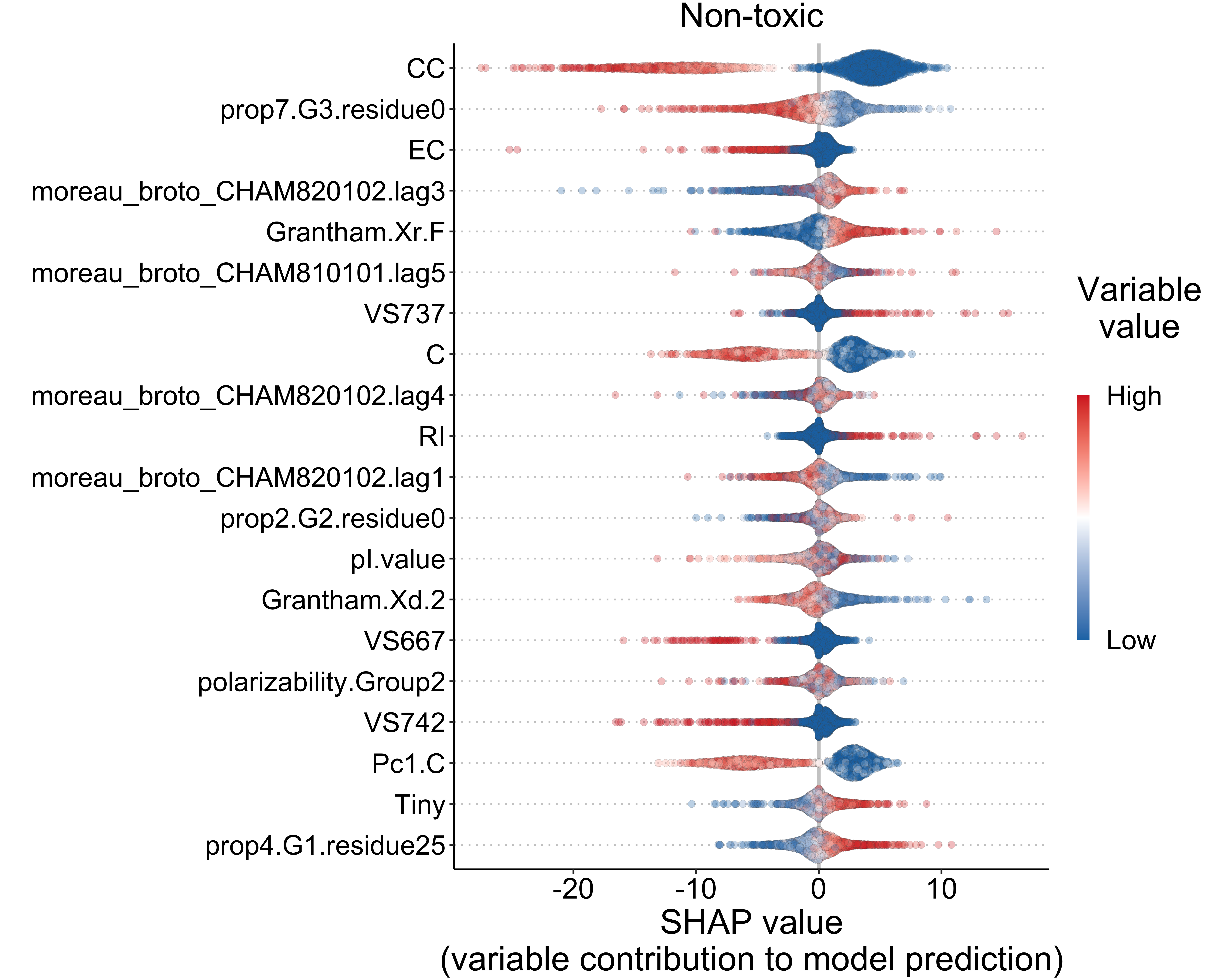
4.3 Multifunctional peptide selection
load(file = paste0("./rdata/tsne_res.RData"))
load(file = paste0("./rdata/var_reduct_mb_train_test_splits.RData"))
tsne_df$mb_predict <- rescale(tsne_df$mb_predict, to = c(0, 100), from = range(mb_data$log_intensity))
tsne_df$mb_predict[tsne_df$mb_predict > 100] <- 100
tsne_df_ <- tsne_df[tsne_df$source == "Validation control" | tsne_df$source == "Validation set", ]
tsne_df_$note[tsne_df_$note == "TAT"] <- NA
tsne_df_$color <- factor(sapply(tsne_df_$note, function(x) if (is.na(x)) 0 else 1))
p <- plot_ly(tsne_df_, x = ~in_vitro_mb_value, y = ~in_vitro_cp_value, z = ~non_tx_prob, text = ~note, color = ~color, colors = c("grey70", "black"), width = 700, height = 600) %>%
add_trace(
marker = list(size = 5, line = list(color = "black", width = 0.5)),
type = "scatter3d", mode = "text+markers"
) %>%
layout(
scene = list(
xaxis = list(
title = "Peptide bound to mNPs (%)",
range = c(0, 100)
),
yaxis = list(
title = "Peptide (pMol / 100K cells)",
type = "log",
ticktext = list(
"", "5", "", "", "", "", "10",
"", "", "", "50", "", "", "", "", "100",
"", "", "", "500", "", "", "", "", "1,000"
),
tickvals = list(
4, 5, 6, 7, 8, 9, 10,
20, 30, 40, 50, 60, 70, 80, 90, 100,
200, 300, 400, 500, 600, 700, 800, 900, 1000
),
range = c(0.63, 3)
),
zaxis = list(
title = "Non-toxic prediction",
range = c(0, 100)
)
),
showlegend = FALSE, autosize = TRUE
)
p4.4 Explanation of HR97 predictions
4.4.1 Melanin binding
h2o.init(nthreads=-1)

dir_path = '/Users/renee/Downloads/melanin_binding'
model_name = 'superlearner_iter_3'
train = pd.read_csv(dir_path + '/whole_data_set/train_set.csv', index_col=0)
X_train = train.iloc[:, :-1]
X_test = pd.read_csv('./other_data/HR97_ml_input.csv', index_col=0).loc[:,X_train.columns]
model = h2o.load_model(dir_path + '/whole_data_set/' + model_name)
def model_predict_(data):
    data = pd.DataFrame(data, columns=X_train.columns)
    h2o_data = h2o.H2OFrame(data)
    res = model.predict(h2o_data)
    res = res.as_data_frame()
    return(res)

np.random.seed(1)
X_train_ = X_train.iloc[np.random.choice(X_train.shape[0], 100, replace=False), :]
explainer = shap.KernelExplainer(model_predict_, X_train_, link='identity')
shap_res = explainer.shap_values(X_test, nsamples=1000)
h2o.remove_all()

exp = shap.Explanation(shap_res * 100 / 3.89063, explainer.expected_value, data=X_test.iloc[0:1, :], \
                       feature_names=X_train.columns)

fig, ax = plt.subplots(figsize=(10, 7))
shap.plots.waterfall(exp[0], max_display=20, show=False)

yticklabels = plt.gca().get_yticklabels()
for i in range(int(len(yticklabels) / 2)):
    label = yticklabels[i]
    label_ = label.get_text().split(' = ')
    if len(label_) > 1:
        yticklabels[i].set_text(' = ' + label_[0])
    yticklabels[int(i + len(yticklabels) / 2)].set_text(' = '.join(label_[::-1]))

plt.gca().set_yticklabels(yticklabels)
fig.subplots_adjust(left=0.33, bottom=0.167, right=0.93, top=0.920)
fig.set_figwidth(10)
fig.set_figheight(7)
plt.text(40, -4.8, 'SHAP value\n(variable contribution to model prediction)',
         horizontalalignment='center', fontsize=14)
plt.show()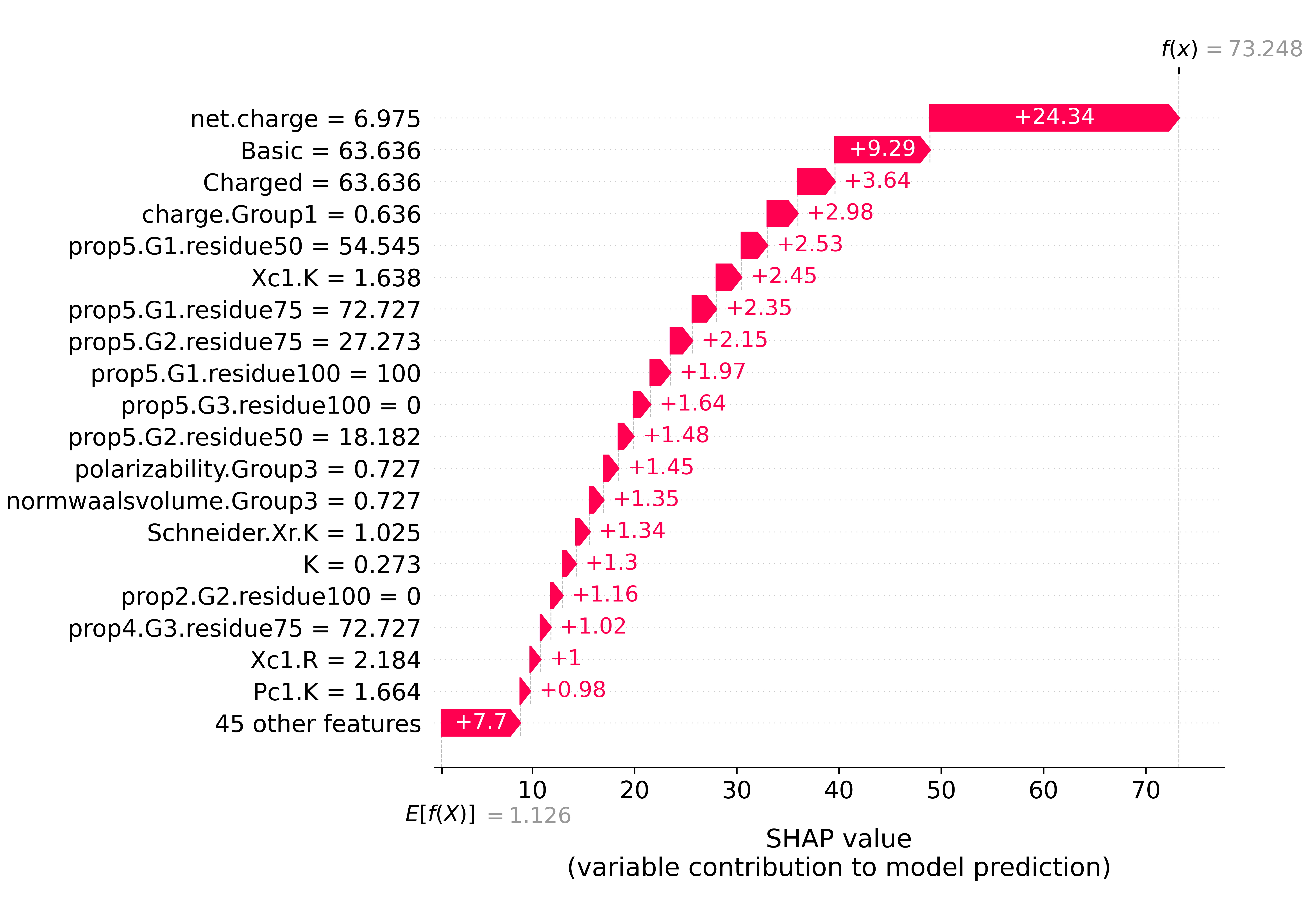
4.4.2 Cell-penetration
h2o.init(nthreads=-1)

dir_path = '/Users/renee/Downloads/cell_penetration'
model_name = 'GBM_model_1669777615732_886421'
train = pd.read_csv(dir_path + '/whole_data_set/train_set.csv', index_col=0)
X_train = train.iloc[:, :-1]
X_test = pd.read_csv('./other_data/HR97_ml_input.csv', index_col=0).loc[:,X_train.columns]
model = h2o.load_model(dir_path + '/whole_data_set/' + model_name)
def model_predict_(data):
    data = pd.DataFrame(data, columns=X_train.columns)
    h2o_data = h2o.H2OFrame(data)
    res = model.predict(h2o_data)
    res = res.as_data_frame().iloc[:,2]
    return(res)

np.random.seed(1)
X_train_ = X_train.iloc[np.random.choice(X_train.shape[0], 100, replace=False), :]
explainer = shap.KernelExplainer(model_predict_, X_train_, link='identity')
shap_res = explainer.shap_values(X_test, nsamples=1000)
h2o.remove_all()

exp = shap.Explanation(shap_res * 100, explainer.expected_value * 100, data=X_test.iloc[0:1, :], \
                       feature_names=X_train.columns)

fig, ax = plt.subplots(figsize=(10, 5))
shap.plots.waterfall(exp[0], max_display=11, show=False)

yticklabels = plt.gca().get_yticklabels()
for i in range(int(len(yticklabels) / 2)):
    label = yticklabels[i]
    label_ = label.get_text().split(' = ')
    if len(label_) > 1:
        yticklabels[i].set_text(' = ' + label_[0])
    yticklabels[int(i + len(yticklabels) / 2)].set_text(' = '.join(label_[::-1]))

plt.gca().set_yticklabels(yticklabels)
fig.subplots_adjust(left=0.32, bottom=0.18, right=0.927, top=0.925)
fig.set_figwidth(10)
fig.set_figheight(5)
plt.text(72, -3.5, 'SHAP value\n(variable contribution to model prediction)',
         horizontalalignment='center', fontsize=14)
plt.show()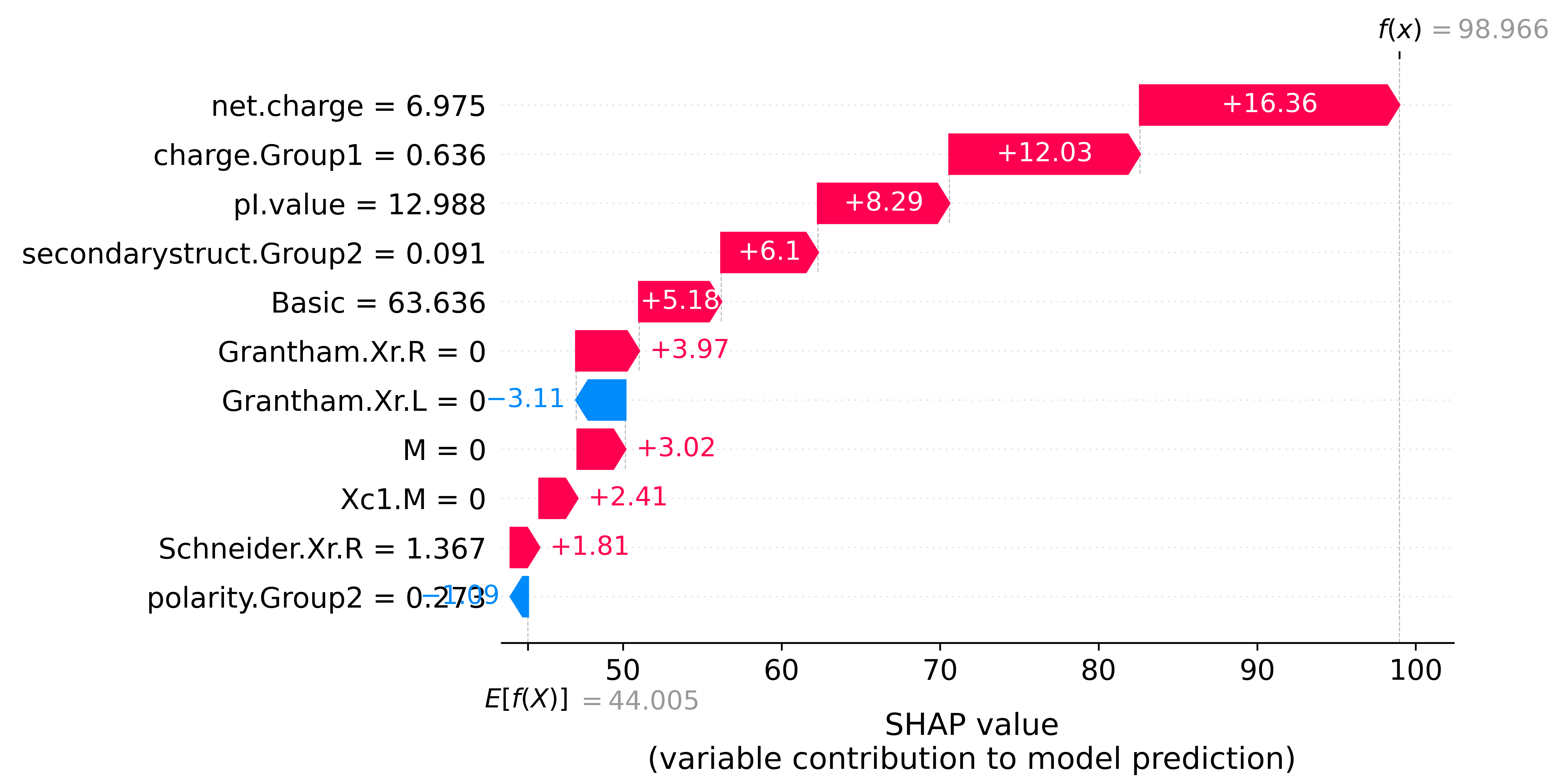
4.4.3 Toxicity
h2o.init(nthreads=-1)

dir_path = '/Users/renee/Downloads/toxicity'
model_name = 'superlearner_iter_3'
train = pd.read_csv(dir_path + '/whole_data_set/train_set.csv', index_col=0)
X_train = train.iloc[:, :-1]
X_test = pd.read_csv('./other_data/HR97_ml_input.csv', index_col=0).loc[:,X_train.columns]
model = h2o.load_model(dir_path + '/whole_data_set/' + model_name)
def model_predict_(data):
    data = pd.DataFrame(data, columns=X_train.columns)
    h2o_data = h2o.H2OFrame(data)
    res = model.predict(h2o_data)
    res = res.as_data_frame().iloc[:,2]
    return(res)

np.random.seed(1)
X_train_ = X_train.iloc[np.random.choice(X_train.shape[0], 100, replace=False), :]
explainer = shap.KernelExplainer(model_predict_, X_train_, link='identity')
shap_res = explainer.shap_values(X_test, nsamples=1000)
h2o.remove_all()

exp = shap.Explanation(shap_res * 100, explainer.expected_value * 100, data=X_test.iloc[0:1, :], \
                       feature_names=X_train.columns)

fig, ax = plt.subplots(figsize=(10, 5))
shap.plots.waterfall(exp[0], max_display=11, show=False)

yticklabels = plt.gca().get_yticklabels()
for i in range(int(len(yticklabels) / 2)):
    label = yticklabels[i]
    label_ = label.get_text().split(' = ')
    if len(label_) > 1:
        yticklabels[i].set_text(' = ' + label_[0])
    yticklabels[int(i + len(yticklabels) / 2)].set_text(' = '.join(label_[::-1]))

plt.gca().set_yticklabels(yticklabels)
fig.subplots_adjust(left=0.395, bottom=0.18, right=0.927, top=0.925)
fig.set_figwidth(10)
fig.set_figheight(5)
plt.text(80, -3.5, 'SHAP value\n(variable contribution to model prediction)',
         horizontalalignment='center', fontsize=14)
plt.show()
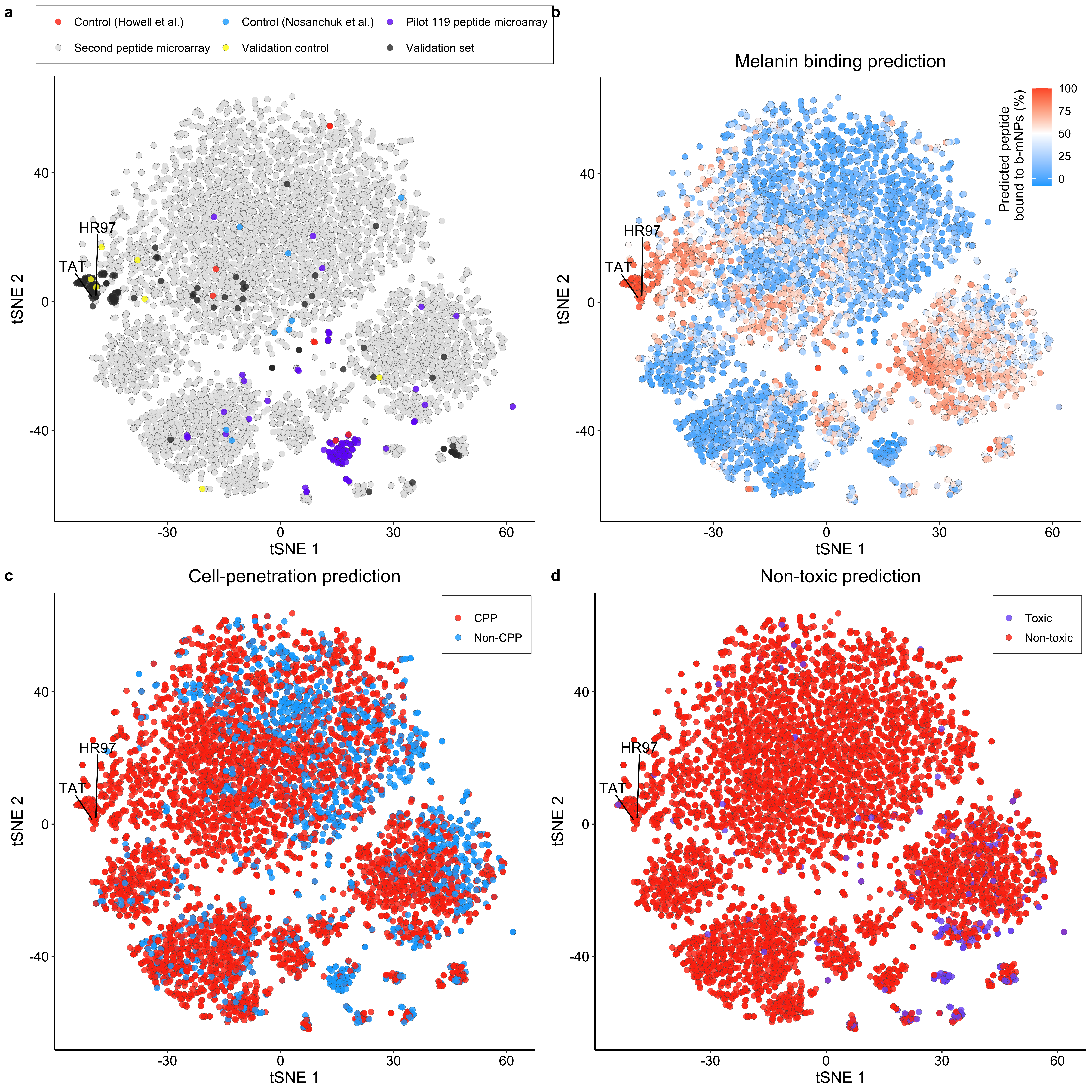
4.5 Peptide design space visualization
p1 <- ggplot(tsne_df, aes(x = `tSNE 1`, y = `tSNE 2`, fill = source)) +
  geom_point(color = "grey30", shape = 21, alpha = 0.8, size = 2.5, stroke = 0.1) +
  geom_text_repel(aes(label = note), color = "black", size = 4.5, nudge_x = -10, nudge_y = 10, point.padding = 0.1, force = 100) +
  scale_fill_manual(values = c("#FF380D", "#0DACFF", "#7134F7", "grey90", "#FEFA0A", "grey20")) +
  theme_bw() +
  theme(
    plot.margin = ggplot2::margin(5, 10, 5, 10),
    plot.background = element_rect(fill = "transparent", color = NA),
    panel.background = element_rect(fill = "transparent"),
    panel.grid.major = element_blank(),
    panel.grid.minor = element_blank(),
    strip.background = element_blank(),
    panel.border = element_blank(),
    axis.line = element_line(color = "black"),
    plot.title = element_text(hjust = 0.5, size = 16),
    axis.title.x = element_text(hjust = 0.5, colour = "black", size = 14),
    axis.title.y = element_text(colour = "black", size = 14),
    axis.text.x = element_text(colour = "black", size = 12),
    axis.text.y = element_text(colour = "black", size = 12),
    legend.title = element_blank(),
    legend.text = element_text(colour = "black", size = 10),
    legend.title.align = 0.5,
    legend.position = "top",
    legend.background = element_rect(fill = "transparent", color = "black", linetype = "solid", size = 0.1)
  ) +
  guides(fill = guide_legend(nrow = 2, byrow = TRUE))

p2 <- ggplot(tsne_df, aes(x = `tSNE 1`, y = `tSNE 2`, fill = mb_predict)) +
  geom_point(color = "grey30", shape = 21, alpha = 0.8, size = 2.5, stroke = 0.1) +
  geom_text_repel(aes(label = note), color = "black", size = 4.5, nudge_x = -10, nudge_y = 10, point.padding = 0.1, force = 100) +
  scale_fill_gradient2(low = "#0DACFF", mid = "white", high = "#FF380D", midpoint = 50) +
  theme_bw() +
  theme(
    plot.margin = ggplot2::margin(5, 10, 5, 10),
    plot.background = element_rect(fill = "transparent", color = NA),
    panel.background = element_rect(fill = "transparent"),
    panel.grid.major = element_blank(),
    panel.grid.minor = element_blank(),
    strip.background = element_blank(),
    panel.border = element_blank(),
    axis.line = element_line(color = "black"),
    plot.title = element_text(hjust = 0.5, size = 16),
    axis.title.x = element_text(hjust = 0.5, colour = "black", size = 14),
    axis.title.y = element_text(colour = "black", size = 14),
    axis.text.x = element_text(colour = "black", size = 12),
    axis.text.y = element_text(colour = "black", size = 12),
    legend.title = element_text(colour = "black", size = 12, angle = 90),
    legend.text = element_text(colour = "black", size = 10),
    legend.title.align = 0.5,
    legend.position = c(0.91, 0.82),
    legend.background = element_blank()
  ) +
  guides(fill = guide_colorbar(
    title = "Predicted peptide \n bound to b-mNPs (%)",
    title.position = "left"
  )) +
  ggtitle("Melanin binding prediction")

p3 <- ggplot(tsne_df, aes(x = `tSNE 1`, y = `tSNE 2`, fill = cpp_predict)) +
  geom_point(color = "grey30", shape = 21, alpha = 0.8, size = 2.5, stroke = 0.1) +
  geom_text_repel(aes(label = note), color = "black", size = 4.5, nudge_x = -10, nudge_y = 10, point.padding = 0.1, force = 100) +
  scale_fill_manual(values = c("#FF380D", "#0DACFF")) +
  theme_bw() +
  theme(
    plot.margin = ggplot2::margin(5, 10, 5, 10),
    plot.background = element_rect(fill = "transparent", color = NA),
    panel.background = element_rect(fill = "transparent"),
    panel.grid.major = element_blank(),
    panel.grid.minor = element_blank(),
    strip.background = element_blank(),
    panel.border = element_blank(),
    axis.line = element_line(color = "black"),
    plot.title = element_text(hjust = 0.5, size = 16),
    axis.title.x = element_text(hjust = 0.5, colour = "black", size = 14),
    axis.title.y = element_text(colour = "black", size = 14),
    axis.text.x = element_text(colour = "black", size = 12),
    axis.text.y = element_text(colour = "black", size = 12),
    legend.title = element_blank(),
    legend.text = element_text(colour = "black", size = 10),
    legend.title.align = 0.5,
    legend.position = c(0.90, 0.93),
    legend.background = element_rect(fill = "transparent", color = "black", linetype = "solid", size = 0.1)
  ) +
  ggtitle("Cell-penetration prediction")

p4 <- ggplot(tsne_df, aes(x = `tSNE 1`, y = `tSNE 2`, fill = tx_predict)) +
  geom_point(color = "grey30", shape = 21, alpha = 0.8, size = 2.5, stroke = 0.1) +
  geom_text_repel(aes(label = note), color = "black", size = 4.5, nudge_x = -10, nudge_y = 10, point.padding = 0.1, force = 100) +
  scale_fill_manual(values = c("#7d5ef7", "#FF380D")) +
  theme_bw() +
  theme(
    plot.margin = ggplot2::margin(5, 5, 5, 5),
    plot.background = element_rect(fill = "transparent", color = NA),
    panel.background = element_rect(fill = "transparent"),
    panel.grid.major = element_blank(),
    panel.grid.minor = element_blank(),
    strip.background = element_blank(),
    panel.border = element_blank(),
    axis.line = element_line(color = "black"),
    plot.title = element_text(hjust = 0.5, size = 16),
    axis.title.x = element_text(hjust = 0.5, colour = "black", size = 14),
    axis.title.y = element_text(colour = "black", size = 14),
    axis.text.x = element_text(colour = "black", size = 12),
    axis.text.y = element_text(colour = "black", size = 12),
    legend.title = element_blank(),
    legend.text = element_text(colour = "black", size = 10),
    legend.title.align = 0.5,
    legend.position = c(0.90, 0.93),
    legend.background = element_rect(fill = "transparent", color = "black", linetype = "solid", size = 0.1)
  ) +
  ggtitle("Non-toxic prediction")
combined <- plot_grid(p1,
plot_grid(NULL, p2, nrow = 2, rel_heights = c(0.08, 0.85)),
p3, p4,
nrow = 2, rel_heights = c(0.48, 0.45),
labels = c("a", "b", "c", "d")
)
sessionInfo()## R version 4.2.2 (2022-10-31)
## Platform: x86_64-apple-darwin17.0 (64-bit)
## Running under: macOS Big Sur ... 10.16
##
## Matrix products: default
## BLAS: /Library/Frameworks/R.framework/Versions/4.2/Resources/lib/libRblas.0.dylib
## LAPACK: /Library/Frameworks/R.framework/Versions/4.2/Resources/lib/libRlapack.dylib
##
## locale:
## [1] en_US.UTF-8/en_US.UTF-8/en_US.UTF-8/C/en_US.UTF-8/en_US.UTF-8
##
## attached base packages:
## [1] stats graphics grDevices utils datasets methods base
##
## other attached packages:
## [1] ggrepel_0.9.1 plotly_4.10.0 cowplot_1.1.1 ggforce_0.3.4
## [5] scales_1.2.1 reshape2_1.4.4 reticulate_1.25 ggbeeswarm_0.6.0
## [9] ggpubr_0.4.0 ggplot2_3.3.6 h2o_3.38.0.2
##
## loaded via a namespace (and not attached):
## [1] httr_1.4.4 sass_0.4.2 tidyr_1.2.0 viridisLite_0.4.1
## [5] jsonlite_1.8.0 here_1.0.1 carData_3.0-5 R.utils_2.12.0
## [9] bslib_0.4.0 assertthat_0.2.1 highr_0.9 vipor_0.4.5
## [13] yaml_2.3.5 pillar_1.8.1 backports_1.4.1 lattice_0.20-45
## [17] glue_1.6.2 digest_0.6.29 ggsignif_0.6.3 polyclip_1.10-0
## [21] colorspace_2.0-3 htmltools_0.5.3 Matrix_1.5-1 R.oo_1.25.0
## [25] plyr_1.8.7 pkgconfig_2.0.3 broom_1.0.0 bookdown_0.28
## [29] purrr_0.3.4 tweenr_2.0.1 tibble_3.1.8 styler_1.8.0
## [33] generics_0.1.3 farver_2.1.1 car_3.1-0 cachem_1.0.6
## [37] withr_2.5.0 lazyeval_0.2.2 cli_3.3.0 magrittr_2.0.3
## [41] evaluate_0.16 R.methodsS3_1.8.2 fansi_1.0.3 R.cache_0.16.0
## [45] MASS_7.3-58.1 rstatix_0.7.0 beeswarm_0.4.0 tools_4.2.2
## [49] data.table_1.14.2 lifecycle_1.0.1 stringr_1.4.1 munsell_0.5.0
## [53] compiler_4.2.2 jquerylib_0.1.4 rlang_1.0.4 grid_4.2.2
## [57] RCurl_1.98-1.8 rstudioapi_0.14 htmlwidgets_1.5.4 crosstalk_1.2.0
## [61] bitops_1.0-7 rmarkdown_2.16 codetools_0.2-18 gtable_0.3.0
## [65] abind_1.4-5 DBI_1.1.3 R6_2.5.1 knitr_1.40
## [69] dplyr_1.0.9 fastmap_1.1.0 utf8_1.2.2 rprojroot_2.0.3
## [73] stringi_1.7.8 Rcpp_1.0.9 vctrs_0.4.1 png_0.1-7
## [77] tidyselect_1.1.2 xfun_0.32session_info.show()## -----
## h2o 3.38.0.2
## matplotlib 3.6.2
## numpy 1.23.5
## pandas 1.5.2
## session_info 1.0.0
## shap 0.41.0
## -----
## Python 3.8.15 | packaged by conda-forge | (default, Nov 22 2022, 09:04:40) [Clang 14.0.6 ]
## macOS-10.16-x86_64-i386-64bit
## -----
## Session information updated at 2023-03-12 23:25