Section 2 Variable reduction
library(Peptides)
library(protr)
library(rlist)
library(ranger)
library(ggplot2)
library(cowplot)
library(scales)
2.1 Methods
- Formula of AIC
\[\begin{equation} AIC = -2\ln(\hat{L}) + 2k, \tag{2.1} \end{equation}\]
\[\begin{equation} \begin{split} \mathrm{where}\:\hat{L}\:\mathrm{is\:the\:maximum\:likelihood\:value,}\\ \mathrm{and}\:k\:\mathrm{is\:the\:number\:of\:parameters.} \end{split} \end{equation}\]
2.1.1 Regression
Likelihood of normal distribution
Assume residuals are normally distributed, then \[\begin{equation} L(\theta) = \prod_{i = 1}^{N} \frac{1}{\sqrt{2\pi\sigma^2}}e^{-\frac{{(\hat{y}_{i} - y_i)}^2}{2\sigma^2}} \tag{2.2} \end{equation}\]
\[\begin{equation} \begin{split} \ln{L(\theta)} & = \sum_{i = 1}^{N} [\ln{(\frac{1}{\sqrt{2\pi\sigma^2}})} - {\frac{{(\hat{y}_{i} - y_i)}^2}{2\sigma^2}}] \\ & = -\frac{N}{2}\ln{(2\pi)} -\frac{N}{2}\ln{(\sigma^2)} - \frac{1}{2\sigma^2}\sum_{i = 1}^{N}{{(\hat{y}_{i} - y_i)}^2.} \\ \end{split} \tag{2.3} \end{equation}\] \(\mathrm{Since}\:{\hat{\sigma}^2} = \frac{\sum_{i = 1}^{N}{{(\hat{y}_{i} - y_i)}^2}}{N} = {MSE},\) \[\begin{equation} \ln{L(\theta)} = -\frac{N}{2}\ln{(MSE)} + C, \mathrm{where}\:C\:\mathrm{is\:a\:constant.} \tag{2.4} \end{equation}\]
- Derived regression AIC
\[\begin{equation} AIC_{reg} = N\ln{(MSE)} + 2k \tag{2.5} \end{equation}\]
2.1.2 Classification
- Likelihood of Bernoulli distribution
\[\begin{equation} L(\theta) = \prod_{i = 1}^{N} [q_{\theta}(y_i = 1)^{y_i}q_{\theta}(y_i = 0)^{1-y_i}] \tag{2.6} \end{equation}\]
\[\begin{equation} \begin{split} \ln{L(\theta)} = \sum_{i = 1}^{N} [y_i\ln{q_{\theta}(y_i = 1)} + (1 - y_i)\ln{q_{\theta}(y_i = 0)}], \end{split} \tag{2.7} \end{equation}\]
\[\begin{equation} \begin{split} \mathrm{where}\:q_{\theta}\:\mathrm{is\:the\:estimated\:probability\:with\:parameters\:\theta}\:\mathrm{and\:}\:y_i \in \{0, 1\} \end{split} \end{equation}\]
- Binary cross-entropy
\[\begin{equation} \begin{split} H_p(q_{\theta}) & = -\frac{1}{N}\sum_{i = 1}^{N} [y_i\log_2{q_{\theta}(y_i = 1)} + (1 - y_i)\log_2{q_{\theta}(y_i = 0)}] \\ & = -\frac{1}{N{\cdot}\ln{2}}\sum_{i = 1}^{N} [y_i\ln{q_{\theta}(y_i = 1)} + (1 - y_i)\ln{q_{\theta}(y_i = 0)}] \end{split} \tag{2.8} \end{equation}\]
- Derived classification AIC
\[\begin{equation} AIC_{clf} = 2{\cdot}\ln{2}{\cdot}N{\cdot}H_p(q_{\theta}) + 2k \tag{2.9} \end{equation}\]
2.1.2.1 Extension to multi-class classification
Generalized likelihood estimation
Assume the classes are one-hot encoded, then we can generalize equation (2.9) to multi-class problems.
\[\begin{equation} L(\theta) = \prod_{i = 1}^{N}\prod_{j = 1}^{M}\hat{y}_{ij}^{y_{ij}} \tag{2.10} \end{equation}\]
\[\begin{equation} \begin{split} \ln{L(\theta)} = \sum_{i = 1}^{N}\sum_{j = 1}^{M}y_{ij}\ln{\hat{y}_{ij}}, \end{split} \tag{2.11} \end{equation}\]
\[\begin{equation} \begin{split} \mathrm{where}\:\hat{y}_{ij}\:\mathrm{is\:the\:estimated\:probability\:of\:class}\:j\:\mathrm{of\:sample\:}i\:\mathrm{and\:}\:y_{ij} \in \{0, 1\} \end{split} \end{equation}\]
- Categorical cross-entropy
\[\begin{equation} H_p(q_{\theta}) = -\frac{1}{N}\sum_{i = 1}^{N}\sum_{j = 1}^{M}y_{ij}\log_2{\hat{y}_{ij}} \tag{2.12} \end{equation}\]
- Derived generalized classification AIC
\[\begin{equation} AIC_{clf} = 2{\cdot}\ln{2}{\cdot}N{\cdot}H_p(q_{\theta}) + 2k \tag{2.13} \end{equation}\]
2.2 ML input generating function
generate_ml_input <- function(fasta_file, label_file, output_file) {
  # --------------
  # Peptides_2.4.4
  # --------------
  # read in fasta file
  peptides <- read.fasta(fasta_file, seqtype = "AA", as.string = TRUE, set.attributes = FALSE)
  # Molecular weight
  weights <- as.matrix(sapply(peptides, function(x) mw(x, monoisotopic = FALSE)))
  colnames(weights) <- "weight"
  # Amino acid composition
  aa.comp <- sapply(peptides, function(x) aaComp(x))
  aa.comp.matrix <- t(sapply(aa.comp, function(x) x[, "Mole%"]))
  # Isoelectric point
  pI.values <- as.matrix(sapply(peptides, function(x) pI(x, pKscale = "EMBOSS")))
  colnames(pI.values) <- "pI.value"
  # Hydrophobicity
  hydrophobicity.values <- as.matrix(sapply(peptides, function(x) hydrophobicity(x, scale = "KyteDoolittle")))
  colnames(hydrophobicity.values) <- "hydrophobicity.value"
  # Net charge at pH 7
  net.charges <- as.matrix(sapply(peptides, function(x) charge(x, pH = 7, pKscale = "EMBOSS")))
  colnames(net.charges) <- "net.charge"
  # Boman index
  boman.indices <- as.matrix(sapply(peptides, function(x) boman(x)))
  colnames(boman.indices) <- "boman.index"
  # combine peptides results
  peptides_res <- data.frame(cbind(weights, aa.comp.matrix, pI.values, hydrophobicity.values, net.charges, boman.indices))

  # -----------
  # protr_1.6-2
  # -----------
  length <- 7
  # read in FASTA file
  sequences <- readFASTA(fasta_file)
  sequences <- sequences[unlist(lapply(sequences, function(x) nchar(x) > 1))]
  # calculate amino acid composition descriptors (dim = 20)
  x1 <- t(sapply(sequences, extractAAC))
  colnames(x1)[colnames(x1) == "Y"] <- "Y_tyrosine"
  # calculate dipeptide composition descriptors (dim = 400)
  x2 <- t(sapply(sequences, extractDC))
  colnames(x2)[colnames(x2) == "NA"] <- "NA_dipeptide"
  # calculate Moreau-Broto autocorrelation descriptors (dim = 8 * (length - 1))
  x3 <- t(sapply(sequences, extractMoreauBroto, nlag = length - 1L))
  colnames(x3) <- paste("moreau_broto", colnames(x3), sep = "_")
  # calculate composition descriptors (dim = 21)
  x4 <- t(sapply(sequences, extractCTDC))
  # calculate transition descriptors (dim = 21)
  x5 <- t(sapply(sequences, extractCTDT))
  # calculate distribution descriptors (dim = 105)
  x6 <- t(sapply(sequences, extractCTDD))
  # calculate conjoint triad descriptors (dim = 343)
  x7 <- t(sapply(sequences, extractCTriad))
  # calculate sequence-order-coupling numbers (dim = 2 * (length - 1))
  x8 <- t(sapply(sequences, extractSOCN, nlag = length - 1L))
  # calculate quasi-sequence-order descriptors (dim = 40 + 2 * (length - 1))
  x9 <- t(sapply(sequences, extractQSO, nlag = length - 1L))
  # calculate pseudo-amino acid composition (dim = 20 + (length - 1))
  x10 <- t(sapply(sequences, extractPAAC, lambda = length - 1L))
  # calculate amphiphilic pseudo-amino acid composition (dim = 20 + 2 * (length - 1))
  x11 <- t(sapply(sequences, extractAPAAC, lambda = length - 1L))
  # combine all of the result datasets
  protr_res <- data.frame(cbind(x1, x2, x3, x4, x5, x6, x7, x8, x9, x10, x11))

  labels <- read.csv(label_file, row.names = 1)
  merge.all <- function(x, ..., by = "row.names") { # https://stackoverflow.com/a/22618297
    L <- list(...)
    for (i in seq_along(L)) {
      x <- merge(x, L[[i]], by = by)
      rownames(x) <- x$Row.names
      x$Row.names <- NULL
    }
    return(x)
  }
  data <- merge.all(peptides_res, protr_res, labels)
  write.csv(data, file = output_file)
}
2.3 AIC functions
#' Mean squared error function
#'
#' @param y_true a factor vector representing true values.
#' @param y_pred a numeric vector or a matrix of predicted values.
#'
#' @return MSE
#'
mse <- function(y_true, y_pred) {
  return(mean((y_true - y_pred)^2))
}
#' Regression AIC
#'
#' @param y_true a factor vector representing true values.
#' @param y_pred a numeric vector or a matrix of predicted values.
#' @param k number of parameters/variables.
#' @param eps a very small value to avoid negative infinitives generated by log(p=0).
#'
#' @return AIC
#'
aic_reg <- function(y_true, y_pred, k, eps = 1e-15) {
mserr <- mse(y_true, y_pred)
if (mserr == 0) mserr <- eps
AIC <- length(y_true) * log(mserr) + 2 * k
return(AIC)
}#' Cross-entropy function
#'
#' @param y_true a factor vector representing true labels.
#' @param y_pred a numeric vector (probabilities of the second class/factor level)
#' or a matrix of predicted probabilities.
#' @param eps a very small value to avoid negative infinitives generated by log(p=0).
#' If the function returns NaN, then increasing eps may solve the issue. Alternatively,
#' As NaN is usually generated in the case of p = 1 - eps = 1, resulting in log(1 - p)
#' = log(0) from binary cross-entropy, the user can pass prediction values as a matrix
#' to calculate categorical cross-entropy instead.
#'
#' @return H, cross-entropy (mean loss per sample)
#'
crossEntropy <- function(y_true, y_pred, eps = 1e-15) {
stopifnot(is.factor(y_true))
y_pred <- pmax(pmin(y_pred, 1 - eps), eps)
n_levels <- nlevels(y_true)
H <- NULL
# Binary classification
if (n_levels == 2 && is.vector(y_pred)) {
y_true <- as.numeric(y_true == levels(y_true)[-1])
H <- -mean(y_true * log2(y_pred) + (1 - y_true) * log2(1 - y_pred))
}
# Multi-class classification
else if (n_levels == ncol(y_pred)) {
y_true <- as.numeric(y_true)
y_true_encoded <- t(sapply(y_true, function(x) {
tmp <- rep(0, n_levels)
tmp[x] <- 1
return(tmp)
}))
H <- -mean(sapply(1:nrow(y_true_encoded), function(x) sum(y_true_encoded[x, ] * log2(y_pred[x, ]))))
}
return(H)
}#' Classification AIC
#'
#' @param y_true a factor vector representing true labels.
#' @param y_pred a numeric vector or a matrix of predicted probabilities.
#' @param k number of parameters/variables.
#' @param ... other parameters to be passed to `crossEntropy()`
#'
#' @return AIC
#'
aic_clf <- function(y_true, y_pred, k, ...) {
H <- crossEntropy(y_true, y_pred, ...)
AIC <- 2 * log(2) * length(y_true) * H + 2 * k
return(AIC)
}2.4 Melanin binding (regression)
2.4.1 Generating ML input
generate_ml_input(
  fasta_file = "./other_data/mb_second_peptide_array.fasta",
  label_file = "./other_data/mb_second_peptide_array_labels.csv",
  output_file = "./data/mb_second_peptide_array_ml_input.csv"
)
2.4.2 Variable importance
set.seed(12)
mb_data <- read.csv("./data/mb_second_peptide_array_ml_input.csv", check.names = FALSE, row.names = 1)
# random shuffle
mb_data <- mb_data[sample(1:nrow(mb_data), replace = FALSE), ]

# train random forest using ranger
ntree <- 100000
predictor_variables <- subset(mb_data, select = -log_intensity)
response_variable <- mb_data$log_intensity
rf <- ranger(
  x = predictor_variables, y = response_variable, num.trees = ntree, importance = "permutation", verbose = TRUE,
  scale.permutation.importance = TRUE, seed = 3, keep.inbag = TRUE
)
save(rf, file = "./rdata/var_reduct_mb_rf.RData")
2.4.3 Variable reduction
load(file = "./rdata/var_reduct_mb_rf.RData")
var_imp <- ranger::importance(rf)
var_imp <- var_imp[order(-var_imp)]
var_imp <- var_imp[var_imp >= 0]

set.seed(12)
mb_data <- read.csv("./data/mb_second_peptide_array_ml_input.csv", check.names = FALSE, row.names = 1)
# random shuffle
mb_data <- mb_data[sample(1:nrow(mb_data), replace = FALSE), ]

ntree <- 1000
var_subset_res <- list()
for (i in 1:length(var_imp)) {
  cat(paste0(i, "\n"))
  predictor_variables <- mb_data[, colnames(mb_data) %in% names(var_imp)[1:i], drop = FALSE]
  response_variable <- mb_data$log_intensity
  rf <- ranger(x = predictor_variables, y = response_variable, num.trees = ntree, importance = "none", verbose = TRUE, seed = 3)
  var_subset_res <- list.append(var_subset_res, list(
    rsq = rf$r.squared,
    aic = aic_reg(
      y_true = response_variable,
      y_pred = rf$predictions,
      k = i
    )
  ))
}
save(var_subset_res, file = "./rdata/var_reduct_mb_var_subset_res.RData")load(file = "./rdata/var_reduct_mb_var_subset_res.RData")
rsq_vec <- unlist(lapply(var_subset_res, function(x) x$rsq))
aic_vec <- unlist(lapply(var_subset_res, function(x) x$aic))
rsq_cutoff <- which.max(rsq_vec)
aic_cutoff <- which.min(aic_vec)
p1_1 <- ggplot(data = data.frame(x = 1:length(rsq_vec), y = rsq_vec), aes(x = x, y = y)) +
geom_point(colour = "black", alpha = 0.3, size = 0.5) +
geom_vline(xintercept = rsq_cutoff, colour = "red", linetype = "dashed") +
scale_x_continuous(breaks = c(1, rsq_cutoff, 200, 400, 600, 735)) +
scale_y_continuous(
breaks = c(0.40, 0.45, 0.50, 0.55),
labels = c("0.40", "0.45", "0.50", "0.55")
) +
theme_bw() +
theme(
plot.margin = unit(c(10, 10, -10, 10), "pt"),
panel.grid.major = element_blank(),
panel.grid.minor = element_blank(),
strip.background = element_blank(),
panel.border = element_blank(),
axis.line = element_line(color = "black"),
plot.title = element_text(hjust = 0.5),
axis.title = element_text(colour = "black"),
axis.text = element_text(colour = "black")
) +
xlab("") +
ylab(expression(italic(R^2))) +
ggtitle("Melanin binding")
p1_2 <- ggplot(data = data.frame(x = 1:length(aic_vec), y = aic_vec), aes(x = x, y = y)) +
geom_point(colour = "black", alpha = 0.3, size = 0.5) +
geom_vline(xintercept = aic_cutoff, colour = "red", linetype = "dashed") +
scale_x_continuous(breaks = c(1, aic_cutoff, 200, 400, 600, 735)) +
scale_y_continuous(
breaks = c(-500, 0, 500, 1000),
labels = c("-500", "0", "500", "1,000")
) +
theme_bw() +
theme(
plot.margin = unit(c(-15, 10, 10, 10), "pt"),
panel.grid.major = element_blank(),
panel.grid.minor = element_blank(),
strip.background = element_blank(),
panel.border = element_blank(),
axis.line = element_line(color = "black"),
plot.title = element_text(hjust = 0.5),
axis.title = element_text(colour = "black"),
axis.text = element_text(colour = "black")
) +
xlab("Number of variables") +
ylab("AIC") +
ggtitle("")
cat(paste0("Maximum R-squared: ", formatC(rsq_vec[rsq_cutoff], format = "f", digits = 3), "\n"))
cat(paste0("R-squared at AIC cutoff: ", formatC(rsq_vec[aic_cutoff], format = "f", digits = 3), "\n"))2.4.4 Generating train-test splits
set.seed(12)
mb_data <- read.csv("./data/mb_second_peptide_array_ml_input.csv", check.names = FALSE, row.names = 1)
# random shuffle
mb_data <- mb_data[sample(1:nrow(mb_data), replace = FALSE), ]

cutoff <- aic_cutoff
load(file = "./rdata/var_reduct_mb_rf.RData")
var_imp <- ranger::importance(rf)
var_imp <- var_imp[order(-var_imp)][1:cutoff]
mb_data <- mb_data[, colnames(mb_data) %in% c(names(var_imp), "log_intensity")]

outer_splits <- list()
n_train <- round(nrow(mb_data) * 0.9)
set.seed(22)
for (i in 1:10) {
  # random shuffle
  mb_data_ <- mb_data[sample(1:nrow(mb_data), replace = FALSE), ]
  outer_train <- mb_data_[1:n_train, ]
  outer_test <- mb_data_[(n_train + 1):nrow(mb_data_), ]
  outer_splits <- list.append(outer_splits, list(train = outer_train, test = outer_test))
}
save(mb_data, outer_splits, file = "./rdata/var_reduct_mb_train_test_splits.RData")
2.5 Cell-penetration (classification)
2.5.1 Generating ML input
generate_ml_input(
  fasta_file = "./other_data/CPP924.fasta",
  label_file = "./other_data/cpp_labels.csv",
  output_file = "./data/cpp_ml_input.csv"
)
2.5.2 Variable importance
set.seed(12)
cpp_data <- read.csv("./data/cpp_ml_input.csv", check.names = FALSE, row.names = 1)
# random shuffle
cpp_data <- cpp_data[sample(1:nrow(cpp_data), replace = FALSE), ]

# train random forest using ranger
ntree <- 100000
predictor_variables <- subset(cpp_data, select = -category)
response_variable <- factor(cpp_data$category, levels = c("non-penetrating", "penetrating"))
rf <- ranger(
  x = predictor_variables, y = response_variable, num.trees = ntree, sample.fraction = rep(0.5, 2),
  importance = "permutation", verbose = TRUE, scale.permutation.importance = TRUE, seed = 3, keep.inbag = TRUE
)
save(rf, file = "./rdata/var_reduct_cpp_rf.RData")
2.5.3 Variable reduction
load(file = "./rdata/var_reduct_cpp_rf.RData")
var_imp <- ranger::importance(rf)
var_imp <- var_imp[order(-var_imp)]
var_imp <- var_imp[var_imp >= 0]

set.seed(12)
cpp_data <- read.csv("./data/cpp_ml_input.csv", check.names = FALSE, row.names = 1)
# random shuffle
cpp_data <- cpp_data[sample(1:nrow(cpp_data), replace = FALSE), ]

ntree <- 1000
var_subset_res <- list()
for (i in 1:length(var_imp)) {
  cat(paste0(i, "\n"))
  predictor_variables <- cpp_data[, colnames(cpp_data) %in% names(var_imp)[1:i], drop = FALSE]
  response_variable <- factor(cpp_data$category, levels = c("non-penetrating", "penetrating"))
  rf <- ranger(
    x = predictor_variables, y = response_variable, num.trees = ntree, importance = "none", verbose = TRUE, seed = 3,
    probability = TRUE
  )
  var_subset_res <- list.append(var_subset_res, list(
    acc = 1 - rf$prediction.error,
    aic = aic_clf(
      y_true = response_variable,
      y_pred = rf$predictions,
      k = i
    )
  ))
}
save(var_subset_res, file = "./rdata/var_reduct_cpp_var_subset_res.RData")load(file = "./rdata/var_reduct_cpp_var_subset_res.RData")
acc_vec <- unlist(lapply(var_subset_res, function(x) x$acc))
aic_vec <- unlist(lapply(var_subset_res, function(x) x$aic))
acc_cutoff <- which.max(acc_vec)
aic_cutoff <- which.min(aic_vec)
p2_1 <- ggplot(data = data.frame(x = 1:length(acc_vec), y = acc_vec), aes(x = x, y = y)) +
geom_point(colour = "black", alpha = 0.3, size = 0.5) +
geom_vline(xintercept = acc_cutoff, colour = "red", linetype = "dashed") +
scale_x_continuous(breaks = c(1, acc_cutoff, 250, 500, 750, 955)) +
scale_y_continuous(
breaks = c(0.88, 0.90, 0.92),
labels = c("0.88", "0.90", "0.92")
) +
theme_bw() +
theme(
plot.margin = unit(c(10, 10, -10, 10), "pt"),
panel.grid.major = element_blank(),
panel.grid.minor = element_blank(),
strip.background = element_blank(),
panel.border = element_blank(),
axis.line = element_line(color = "black"),
plot.title = element_text(hjust = 0.5),
axis.title = element_text(colour = "black"),
axis.text = element_text(colour = "black")
) +
xlab("") +
ylab("Accuracy") +
ggtitle("Cell-penetration")
p2_2 <- ggplot(data = data.frame(x = 1:length(aic_vec), y = aic_vec), aes(x = x, y = y)) +
geom_point(colour = "black", alpha = 0.3, size = 0.5) +
geom_vline(xintercept = aic_cutoff, colour = "red", linetype = "dashed") +
scale_x_continuous(breaks = c(aic_cutoff, 250, 500, 750, 955)) +
scale_y_continuous(
breaks = c(500, 1000, 1500, 2000, 2500),
labels = c("500", "1,000", "1,500", "2,000", "2,500")
) +
theme_bw() +
theme(
plot.margin = unit(c(-15, 10, 10, 10), "pt"),
panel.grid.major = element_blank(),
panel.grid.minor = element_blank(),
strip.background = element_blank(),
panel.border = element_blank(),
axis.line = element_line(color = "black"),
plot.title = element_text(hjust = 0.5),
axis.title = element_text(colour = "black"),
axis.text = element_text(colour = "black")
) +
xlab("Number of variables") +
ylab("AIC") +
ggtitle("")
cat(paste0("Maximum accuracy: ", formatC(acc_vec[acc_cutoff], format = "f", digits = 3), "\n"))
cat(paste0("Accuracy at AIC cutoff: ", formatC(acc_vec[aic_cutoff], format = "f", digits = 3), "\n"))2.5.4 Generating train-test splits
set.seed(12)
cpp_data <- read.csv("./data/cpp_ml_input.csv", check.names = FALSE, row.names = 1)
# random shuffle
cpp_data <- cpp_data[sample(1:nrow(cpp_data), replace = FALSE), ]

cutoff <- aic_cutoff
load(file = "./rdata/var_reduct_cpp_rf.RData")
var_imp <- ranger::importance(rf)
var_imp <- var_imp[order(-var_imp)][1:cutoff]
cpp_data <- cpp_data[, colnames(cpp_data) %in% c(names(var_imp), "category")]

outer_splits <- list()
n_train <- round(nrow(cpp_data) * 0.9)
set.seed(22)
for (i in 1:10) {
  # random shuffle
  cpp_data_ <- cpp_data[sample(1:nrow(cpp_data), replace = FALSE), ]
  outer_train <- cpp_data_[1:n_train, ]
  outer_test <- cpp_data_[(n_train + 1):nrow(cpp_data_), ]
  outer_splits <- list.append(outer_splits, list(train = outer_train, test = outer_test))
}
save(cpp_data, outer_splits, file = "./rdata/var_reduct_cpp_train_test_splits.RData")
2.6 Toxicity (classification)
2.6.1 Generating ML input
generate_ml_input(
  fasta_file = "./other_data/toxicity.fasta",
  label_file = "./other_data/tx_labels.csv",
  output_file = "./data/tx_ml_input.csv"
)
2.6.2 Variable importance
set.seed(12)
tx_data <- read.csv("./data/tx_ml_input.csv", check.names = FALSE, row.names = 1)
# random shuffle
tx_data <- tx_data[sample(1:nrow(tx_data), replace = FALSE), ]
# train random forest using ranger
ntree <- 100000
predictor_variables <- subset(tx_data, select = -category)
response_variable <- factor(tx_data$category, levels = c("non-toxic", "toxic"))
rf <- ranger(
  x = predictor_variables, y = response_variable, num.trees = ntree, sample.fraction = rep(0.5, 2),
  importance = "permutation", verbose = TRUE, scale.permutation.importance = TRUE, seed = 3, keep.inbag = TRUE
)
save(rf, file = "./rdata/var_reduct_tx_rf.RData")
2.6.3 Variable reduction
load(file = "./rdata/var_reduct_tx_rf.RData")
var_imp <- ranger::importance(rf)
var_imp <- var_imp[order(-var_imp)]
var_imp <- var_imp[var_imp >= 0]

set.seed(12)
tx_data <- read.csv("./data/tx_ml_input.csv", check.names = FALSE, row.names = 1)
# random shuffle
tx_data <- tx_data[sample(1:nrow(tx_data), replace = FALSE), ]

ntree <- 1000
var_subset_res <- list()
for (i in 1:length(var_imp)) {
  cat(paste0(i, "\n"))
  predictor_variables <- tx_data[, colnames(tx_data) %in% names(var_imp)[1:i], drop = FALSE]
  response_variable <- factor(tx_data$category, levels = c("non-toxic", "toxic"))
  rf <- ranger(
    x = predictor_variables, y = response_variable, num.trees = ntree, importance = "none", verbose = TRUE, seed = 3,
    probability = TRUE
  )
  var_subset_res <- list.append(var_subset_res, list(
    acc = 1 - rf$prediction.error,
    aic = aic_clf(
      y_true = response_variable,
      y_pred = rf$predictions,
      k = i
    )
  ))
}
save(var_subset_res, file = "./rdata/var_reduct_tx_var_subset_res.RData")load(file = "./rdata/var_reduct_tx_var_subset_res.RData")
acc_vec <- unlist(lapply(var_subset_res, function(x) x$acc))
aic_vec <- unlist(lapply(var_subset_res, function(x) x$aic))
acc_cutoff <- which.max(acc_vec)
aic_cutoff <- which.min(aic_vec)
p3_1 <- ggplot(data = data.frame(x = 1:length(acc_vec), y = acc_vec), aes(x = x, y = y)) +
geom_point(colour = "black", alpha = 0.3, size = 0.5) +
geom_vline(xintercept = acc_cutoff, colour = "red", linetype = "dashed") +
scale_x_continuous(
breaks = c(1, acc_cutoff, 300, 600, 900, 1076),
labels = c("1", "148", "300", "600", "900", "1,076")
) +
scale_y_continuous(
breaks = c(0.91, 0.92, 0.93, 0.94, 0.95, 0.96),
labels = c("0.91", "0.92", "0.93", "0.94", "0.95", "0.96")
) +
theme_bw() +
theme(
plot.margin = unit(c(10, 10, -10, 10), "pt"),
panel.grid.major = element_blank(),
panel.grid.minor = element_blank(),
strip.background = element_blank(),
panel.border = element_blank(),
axis.line = element_line(color = "black"),
plot.title = element_text(hjust = 0.5),
axis.title = element_text(colour = "black"),
axis.text = element_text(colour = "black")
) +
xlab("") +
ylab("Accuracy") +
ggtitle("Toxicity")
p3_2 <- ggplot(data = data.frame(x = 1:length(aic_vec), y = aic_vec), aes(x = x, y = y)) +
geom_point(colour = "black", alpha = 0.3, size = 0.5) +
geom_vline(xintercept = aic_cutoff, colour = "red", linetype = "dashed") +
scale_x_continuous(
breaks = c(aic_cutoff, 300, 600, 900, 1076),
labels = c("56", "300", "600", "900", "1,076")
) +
scale_y_continuous(
breaks = c(2000, 3000, 4000, 5000, 6000, 7000),
labels = c("2,000", "3,000", "4,000", "5,000", "6,000", "7,000")
) +
theme_bw() +
theme(
plot.margin = unit(c(-15, 10, 10, 10), "pt"),
panel.grid.major = element_blank(),
panel.grid.minor = element_blank(),
strip.background = element_blank(),
panel.border = element_blank(),
axis.line = element_line(color = "black"),
plot.title = element_text(hjust = 0.5),
axis.title = element_text(colour = "black"),
axis.text = element_text(colour = "black")
) +
xlab("Number of variables") +
ylab("AIC") +
ggtitle("")
cat(paste0("Maximum accuracy: ", formatC(acc_vec[acc_cutoff], format = "f", digits = 3), "\n"))
cat(paste0("Accuracy at AIC cutoff: ", formatC(acc_vec[aic_cutoff], format = "f", digits = 3), "\n"))2.6.4 Generating train-test splits
set.seed(12)
tx_data <- read.csv("./data/tx_ml_input.csv", check.names = FALSE, row.names = 1)
# random shuffle
tx_data <- tx_data[sample(1:nrow(tx_data), replace = FALSE), ]
# convert category so that positive class represents non-toxic
# for evaluation metrics that focus on true positives more than
# true negatives
tx_data$category <- as.factor(sapply(tx_data$category, function(x) if (x == "non-toxic") 1 else 0))

cutoff <- aic_cutoff
load(file = "./rdata/var_reduct_tx_rf.RData")
var_imp <- ranger::importance(rf)
var_imp <- var_imp[order(-var_imp)][1:cutoff]
tx_data <- tx_data[, colnames(tx_data) %in% c(names(var_imp), "category")]

outer_splits <- list()
n_train <- round(nrow(tx_data) * 0.9)
set.seed(22)
for (i in 1:10) {
  # random shuffle
  tx_data_ <- tx_data[sample(1:nrow(tx_data), replace = FALSE), ]
  outer_train <- tx_data_[1:n_train, ]
  outer_test <- tx_data_[(n_train + 1):nrow(tx_data_), ]
  outer_splits <- list.append(outer_splits, list(train = outer_train, test = outer_test))
}
save(tx_data, outer_splits, file = "./rdata/var_reduct_tx_train_test_splits.RData")
2.7 Plotting
p_combined <- plot_grid(p1_1, p2_1, p3_1,
  p1_2, p2_2, p3_2,
  nrow = 2,
  labels = c("a", "b", "c", "", "", ""),
  align = "v"
)
p_combined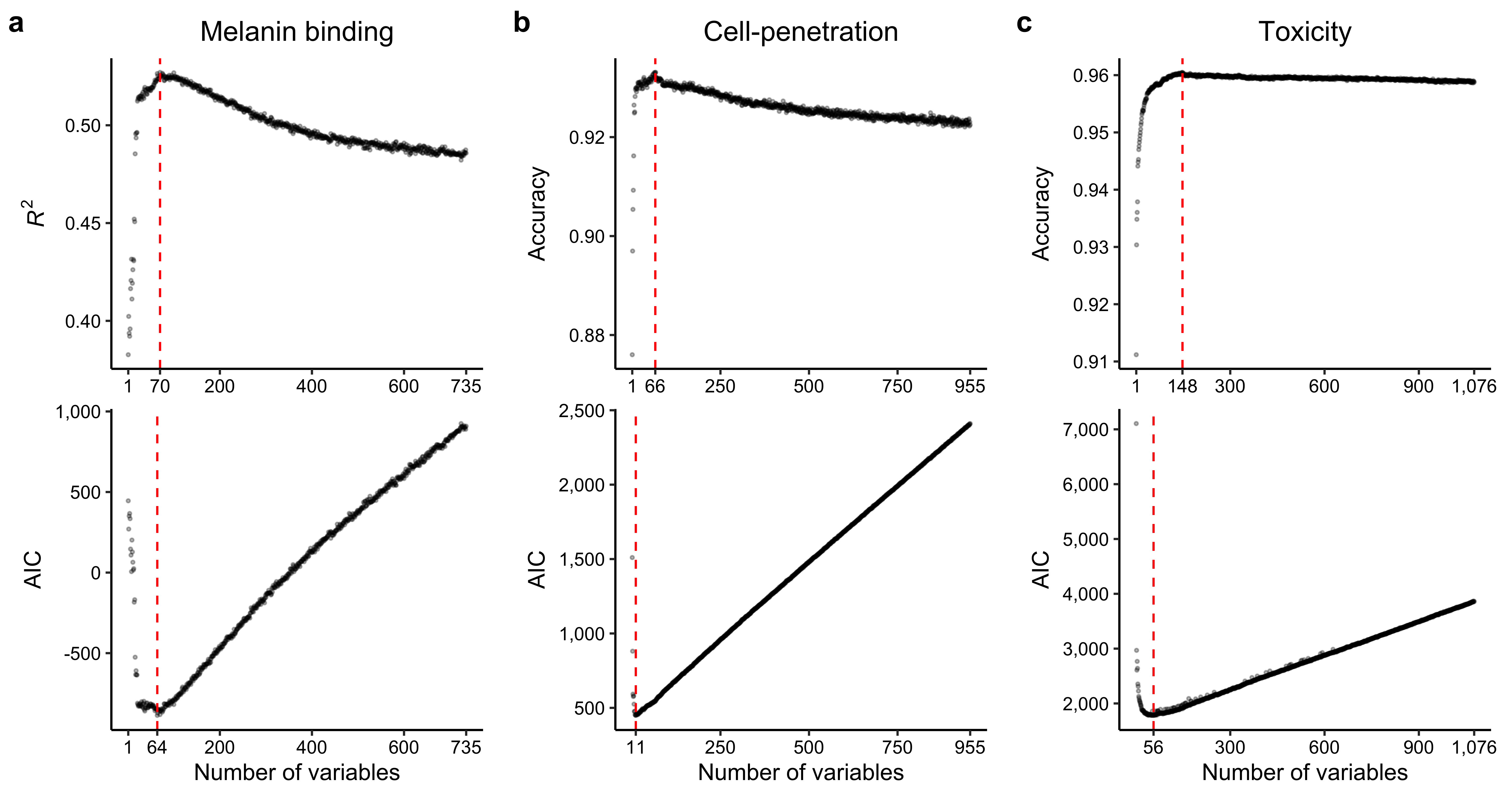
sessionInfo()## R version 4.2.2 (2022-10-31)
## Platform: x86_64-apple-darwin17.0 (64-bit)
## Running under: macOS Big Sur ... 10.16
##
## Matrix products: default
## BLAS: /Library/Frameworks/R.framework/Versions/4.2/Resources/lib/libRblas.0.dylib
## LAPACK: /Library/Frameworks/R.framework/Versions/4.2/Resources/lib/libRlapack.dylib
##
## locale:
## [1] en_US.UTF-8/en_US.UTF-8/en_US.UTF-8/C/en_US.UTF-8/en_US.UTF-8
##
## attached base packages:
## [1] stats graphics grDevices utils datasets methods base
##
## other attached packages:
## [1] scales_1.2.1 cowplot_1.1.1 ggplot2_3.3.6 ranger_0.14.1 rlist_0.4.6.2
## [6] protr_1.6-2 Peptides_2.4.4
##
## loaded via a namespace (and not attached):
## [1] styler_1.8.0 tidyselect_1.1.2 xfun_0.32 bslib_0.4.0
## [5] purrr_0.3.4 lattice_0.20-45 colorspace_2.0-3 vctrs_0.4.1
## [9] generics_0.1.3 htmltools_0.5.3 yaml_2.3.5 utf8_1.2.2
## [13] rlang_1.0.4 R.oo_1.25.0 jquerylib_0.1.4 pillar_1.8.1
## [17] withr_2.5.0 glue_1.6.2 DBI_1.1.3 R.utils_2.12.0
## [21] R.cache_0.16.0 lifecycle_1.0.1 stringr_1.4.1 munsell_0.5.0
## [25] gtable_0.3.0 R.methodsS3_1.8.2 codetools_0.2-18 evaluate_0.16
## [29] knitr_1.40 fastmap_1.1.0 fansi_1.0.3 highr_0.9
## [33] Rcpp_1.0.9 cachem_1.0.6 jsonlite_1.8.0 digest_0.6.29
## [37] stringi_1.7.8 bookdown_0.28 dplyr_1.0.9 grid_4.2.2
## [41] cli_3.3.0 tools_4.2.2 magrittr_2.0.3 sass_0.4.2
## [45] tibble_3.1.8 pkgconfig_2.0.3 Matrix_1.5-1 data.table_1.14.2
## [49] assertthat_0.2.1 rmarkdown_2.16 rstudioapi_0.14 R6_2.5.1
## [53] compiler_4.2.2