Section 4 Model comparisons

4.1 Known antigen score comparisons

In R:

library(ggplot2)
library(reshape2)
library(ggdist)
library(gghalves)
library(cowplot)

pv_scores <- read.csv("./other_data/pv_known_antigen_scores.csv", row.names = 1)
pv_unl_scores <- read.csv("./other_data/pv_unlabeled_protein_scores.csv", row.names = 1)
pv_scores$label <- 2
pv_unl_scores$label <- 1
data_ <- melt(rbind(pv_scores, pv_unl_scores), id.vars = "label")
data_$variable <- factor(data_$variable, levels = c(
  "pf_single_model",
  "pv_single_model", "pv_pf_pos",
  "pfpv_combined_model",
  "pv_pf_unl"
))
data_$label[data_$value < 0.5 & data_$label == 1] <- 0
set.seed(12)
p1 <- ggplot(data_, aes(x = variable, y = value)) +
  geom_hline(yintercept = 0.5, color = "grey70", linetype = "dashed") +
  stat_halfeye(aes(fill = factor(label, levels = c(2, 1, 0))),
    slab_color = "black",
    slab_linewidth = 0.2, adjust = 0.5, width = 0.5, .width = 0,
    justification = -0.2, point_colour = NA, alpha = 0.6, normalize = "all"
  ) +
  geom_boxplot(aes(fill = factor(label, levels = c(2, 1, 0))),
    width = 0.2, outlier.color = NA,
    lwd = 0.3, show.legend = FALSE, alpha = 0.6, color = "black"
  ) +
  geom_half_point(
    data = data_[data_$label == 2, ], fill = "#FCB40A", side = "l",
    range_scale = 0.3, alpha = 0.8, shape = 21, color = "black", stroke = 0.1, size = 2
  ) +
  scale_fill_manual(
    name = "", values = c("#FCB40A", "#FF007F", "#0080FF"), breaks = c(2, 1, 0),
    labels = c("Known antigen", "Predicted antigen", "Predicted non-antigen")
  ) +
  scale_color_manual(
    name = "", values = c("#FCB40A", "#FF007F", "#0080FF"), breaks = c(2, 1, 0),
    labels = c("Known antigen", "Predicted antigen", "Predicted non-antigen")
  ) +
  coord_flip() +
  scale_x_discrete(
    breaks = c(
      "pf_single_model", "pv_single_model", "pv_pf_pos",
      "pfpv_combined_model", "pv_pf_unl"
    ),
    labels = c(
      "Heterologous model", "Autologous model",
      "Autologous with\n heterologous positives model",
      "Combined model",
      "Autologous with\n heterologous unlabeled model"
    ),
    limits = rev
  ) +
  theme_bw() +
  theme(
    panel.grid.major = element_blank(),
    panel.grid.minor = element_blank(),
    axis.title.x = element_text(colour = "black"),
    axis.title.y = element_blank(),
    axis.text = element_text(colour = "black"),
    plot.title = element_text(hjust = 0.5, colour = "black"),
    plot.margin = ggplot2::margin(5, 5, 5, 5, "pt"),
    legend.position = "none"
  ) +
  ylim(0, 1) +
  ylab("Score (proportion of votes)")

legend <- get_legend(p2 +
  theme(
    legend.direction = "horizontal",
    legend.position = "bottom",
    legend.title = element_blank()
  ) +
  guides(fill = guide_legend(title = "")))

pf_scores <- read.csv("./other_data/pf_known_antigen_scores.csv", row.names = 1)
pf_unl_scores <- read.csv("./other_data/pf_unlabeled_protein_scores.csv", row.names = 1)
pf_scores$label <- 2
pf_unl_scores$label <- 1
data_ <- melt(rbind(pf_scores, pf_unl_scores), id.vars = "label")
data_$variable <- factor(data_$variable, levels = c(
  "pv_single_model",
  "pf_single_model", "pf_pv_pos",
  "pfpv_combined_model",
  "pf_pv_unl"
))
data_$label[data_$value < 0.5 & data_$label == 1] <- 0
set.seed(12)
p2 <- ggplot(data_, aes(x = variable, y = value)) +
  geom_hline(yintercept = 0.5, color = "grey70", linetype = "dashed") +
  stat_halfeye(aes(fill = factor(label, levels = c(2, 1, 0))),
    slab_color = "black",
    slab_linewidth = 0.2, adjust = 0.5, width = 0.5, .width = 0,
    justification = -0.2, point_colour = NA, alpha = 0.6, normalize = "all"
  ) +
  geom_boxplot(aes(fill = factor(label, levels = c(2, 1, 0))),
    width = 0.2, outlier.color = NA,
    lwd = 0.3, show.legend = FALSE, alpha = 0.6, color = "black"
  ) +
  geom_half_point(
    data = data_[data_$label == 2, ], fill = "#FCB40A", side = "l",
    range_scale = 0.3, alpha = 0.8, shape = 21, color = "black", stroke = 0.1, size = 2
  ) +
  scale_fill_manual(
    name = "", values = c("#FCB40A", "#FF007F", "#0080FF"), breaks = c(2, 1, 0),
    labels = c("Known antigen", "Predicted antigen", "Predicted non-antigen")
  ) +
  scale_color_manual(
    name = "", values = c("#FCB40A", "#FF007F", "#0080FF"), breaks = c(2, 1, 0),
    labels = c("Known antigen", "Predicted antigen", "Predicted non-antigen")
  ) +
  coord_flip() +
  scale_x_discrete(
    breaks = c(
      "pv_single_model", "pf_single_model", "pf_pv_pos",
      "pfpv_combined_model", "pf_pv_unl"
    ),
    labels = c(
      "Heterologous model", "Autologous model",
      "Autologous with\n heterologous positives model",
      "Combined model",
      "Autologous with\n heterologous unlabeled model"
    ),
    limits = rev
  ) +
  theme_bw() +
  theme(
    panel.grid.major = element_blank(),
    panel.grid.minor = element_blank(),
    axis.title.x = element_text(colour = "black"),
    axis.title.y = element_blank(),
    axis.text = element_text(colour = "black"),
    plot.title = element_text(hjust = 0.5, colour = "black"),
    plot.margin = ggplot2::margin(5, 5, 5, 5, "pt"),
    legend.title = element_blank(),
    legend.text = element_text(colour = "black"),
    legend.position = "none"
  ) +
  ylim(0, 1) +
  ylab("Score (proportion of votes)")

p_combined <- plot_grid(p1, p2, plot_grid(NULL, legend, rel_widths = c(0.2, 0.8)),
  ncol = 2,
  rel_heights = c(1, 0.1), labels = c("a", "b", "", "")
)
p_combined

png(file = "./figures/Fig 2.png", width = 7500, height = 4000, res = 600)
print(p_combined)
dev.off()

pdf(file = "../figures/Fig 2.pdf", width = 13, height = 7)
print(p_combined)
dev.off()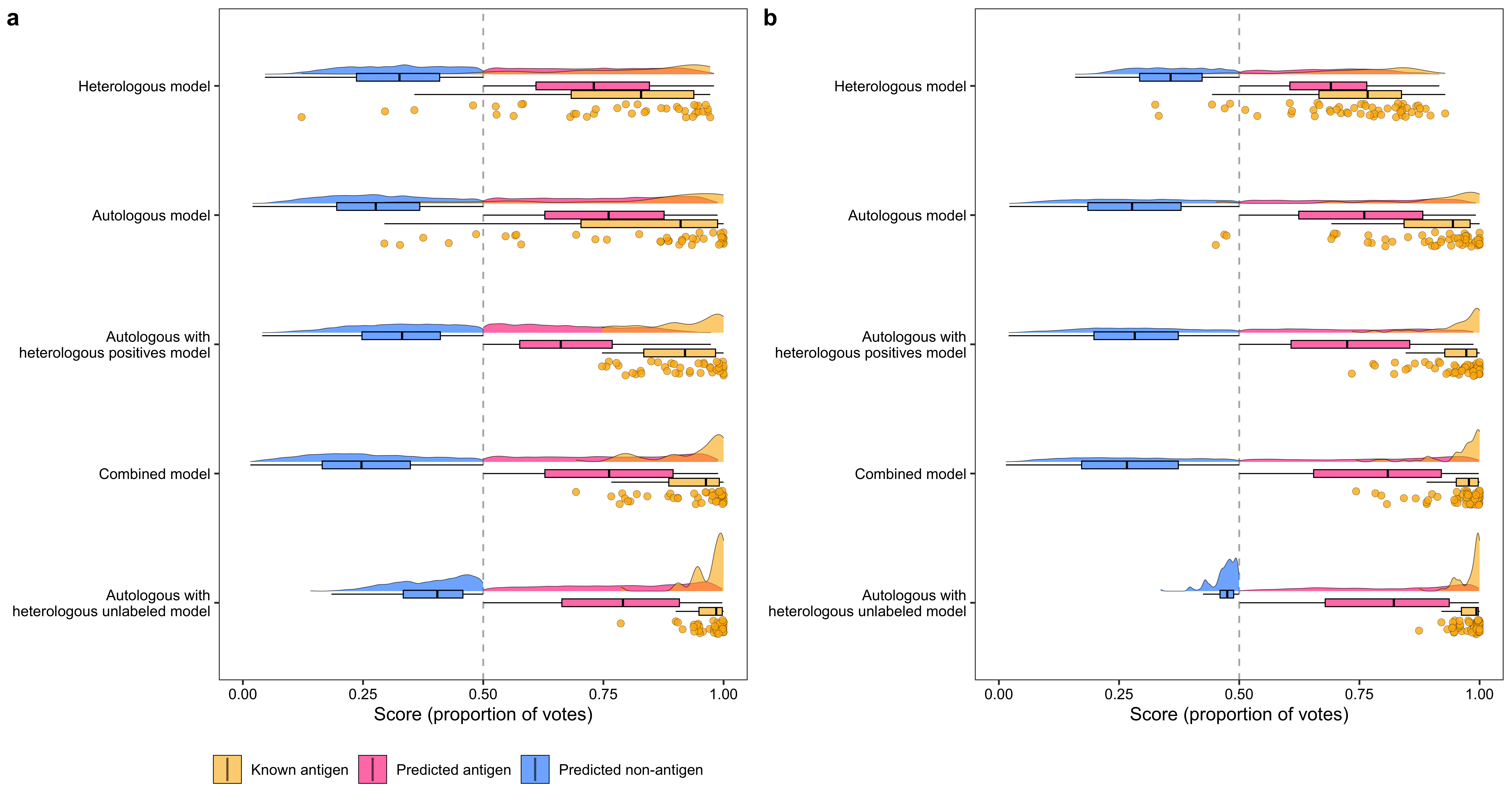

4.2 Known antigen prediction summary

In R:

library(pracma)
library(ggsci)

pv_scores <- read.csv("./other_data/pv_known_antigen_scores.csv", row.names = 1)
pv_unl_scores <- read.csv("./other_data/pv_unlabeled_protein_scores.csv", row.names = 1)
pv_scores$label <- 1
pv_unl_scores$label <- 0
pv_all <- rbind(pv_scores, pv_unl_scores)

data <- data.frame(
  "antigen_label" = pv_all$label,
  "Heterologous model" = pv_all$pf_single_model,
  "Autologous model" = pv_all$pv_single_model,
  "Autologous with heterologous positives model" = pv_all$pv_pf_pos,
  "Combined model" = pv_all$pfpv_combined_model,
  "Autologous with heterologous unlabeled model" = pv_all$pv_pf_unl,
  check.names = FALSE
)

# Calculate percent rank for labeled positives
model_names <- c()
x <- c()
percent_rank <- c()
auc <- c()
for (model in colnames(data)[-1]) {
  data_ <- data[c("antigen_label", model)]
  percent_rank_ <- (rank(data_[[model]]) / nrow(data))[data$antigen_label == 1]
  percent_rank <- c(percent_rank, percent_rank_[order(-percent_rank_)])
  data_ <- data_[data$antigen_label == 1, ]
  data_ <- data_[order(-percent_rank_), ]
  x_ <- 1:nrow(data_) / nrow(data_)
  x <- c(x, x_)
  model_names <- c(model_names, rep(model, nrow(data_)))
  auc <- c(auc, round(trapz(c(0, x_, 1), c(1, percent_rank_, 0)), 2))
  cat(paste0("EPR: ", sum(data_[[model]] >= 0.5) / nrow(data_), "\n"))
}
names(auc) <- colnames(data)[-1]

res <- data.frame(model = model_names, x = x, percent_rank = percent_rank)

p1 <- ggplot(res, aes(x = x, y = `percent_rank`, group = model)) +
  geom_hline(yintercept = 0.5, linetype = "dashed", color = "grey50") +
  geom_line(linewidth = 0.1, color = "grey30") +
  geom_point(aes(fill = model),
    size = 2.2, shape = 21, color = "grey30", stroke = 0.1,
    alpha = 0.8
  ) +
  scale_fill_jco(
    breaks = colnames(data)[-1][order(-auc)],
    labels = sapply(colnames(data)[-1][order(-auc)], function(x) {
      paste0(
        x, " (AUC = ",
        auc[x], ")"
      )
    })
  ) +
  theme_bw() +
  theme(
    panel.grid.major = element_blank(),
    panel.grid.minor = element_blank(),
    axis.title = element_text(colour = "black"),
    axis.text = element_text(colour = "black"),
    plot.title = element_text(hjust = 0.5, colour = "black"),
    legend.title = element_text(hjust = 0.5, colour = "black", angle = 0),
    legend.text = element_text(colour = "black"),
    legend.position = c(0.34, 0.16),
    legend.background = element_blank(),
    legend.key = element_rect(colour = "transparent", fill = "transparent")
  ) +
  labs(fill = "") +
  ylim(0, 1) +
  xlab("Ranked known antigens (scaled)") +
  ylab("Percent rank")

pf_scores <- read.csv("./other_data/pf_known_antigen_scores.csv", row.names = 1)
pf_unl_scores <- read.csv("./other_data/pf_unlabeled_protein_scores.csv", row.names = 1)
pf_scores$label <- 1
pf_unl_scores$label <- 0
pf_all <- rbind(pf_scores, pf_unl_scores)

data <- data.frame(
  "antigen_label" = pf_all$label,
  "Heterologous model" = pf_all$pv_single_model,
  "Autologous model" = pf_all$pf_single_model,
  "Autologous with heterologous positives model" = pf_all$pf_pv_pos,
  "Combined model" = pf_all$pfpv_combined_model,
  "Autologous with heterologous unlabeled model" = pf_all$pf_pv_unl,
  check.names = FALSE
)

# Calculate percent rank for labeled positives
model_names <- c()
x <- c()
percent_rank <- c()
auc <- c()
for (model in colnames(data)[-1]) {
  data_ <- data[c("antigen_label", model)]
  percent_rank_ <- (rank(data_[[model]]) / nrow(data))[data$antigen_label == 1]
  percent_rank <- c(percent_rank, percent_rank_[order(-percent_rank_)])
  data_ <- data_[data$antigen_label == 1, ]
  data_ <- data_[order(-percent_rank_), ]
  x_ <- 1:nrow(data_) / nrow(data_)
  x <- c(x, x_)
  model_names <- c(model_names, rep(model, nrow(data_)))
  auc <- c(auc, round(trapz(c(0, x_, 1), c(1, percent_rank_, 0)), 2))
  cat(paste0("EPR: ", sum(data_[[model]] >= 0.5) / nrow(data_), "\n"))
}
names(auc) <- colnames(data)[-1]

res <- data.frame(model = model_names, x = x, percent_rank = percent_rank)

p2 <- ggplot(res, aes(x = x, y = `percent_rank`, group = model)) +
  geom_hline(yintercept = 0.5, linetype = "dashed", color = "grey50") +
  geom_line(linewidth = 0.1, color = "grey30") +
  geom_point(aes(fill = model),
    size = 2.2, shape = 21, color = "grey30", stroke = 0.1,
    alpha = 0.8
  ) +
  scale_fill_jco(
    breaks = colnames(data)[-1][order(-auc)],
    labels = sapply(colnames(data)[-1][order(-auc)], function(x) {
      paste0(
        x, " (AUC = ",
        auc[x], ")"
      )
    })
  ) +
  theme_bw() +
  theme(
    panel.grid.major = element_blank(),
    panel.grid.minor = element_blank(),
    axis.title = element_text(colour = "black"),
    axis.text = element_text(colour = "black"),
    plot.title = element_text(hjust = 0.5, colour = "black"),
    legend.title = element_text(hjust = 0.5, colour = "black", angle = 0),
    legend.text = element_text(colour = "black"),
    legend.position = c(0.34, 0.16),
    legend.background = element_blank(),
    legend.key = element_rect(colour = "transparent", fill = "transparent")
  ) +
  labs(fill = "") +
  ylim(0, 1) +
  xlab("Ranked known antigens (scaled)") +
  ylab("Percent rank")

p_combined <- plot_grid(p1, p2, nrow = 1, labels = c("a", "b"))
p_combined

png(file = "./figures/Supplementary Fig 6.png", width = 7600, height = 3500, res = 600)
print(p_combined)
dev.off()

pdf(file = "../supplementary_figures/Supplementary Fig 6.pdf", width = 15.2, height = 7)
print(p_combined)
dev.off()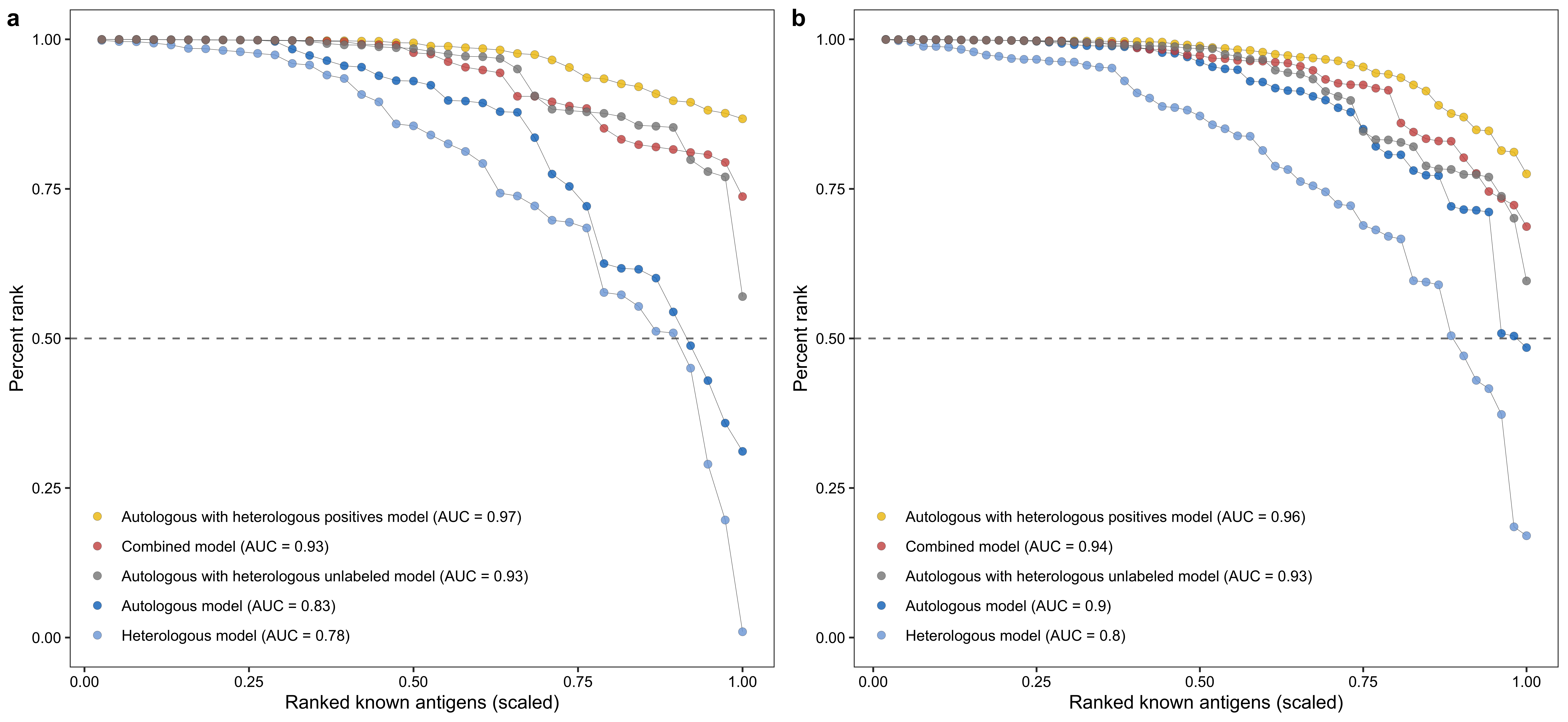

4.3 Score and species association

In R:

library(scales)
library(rlist)
library(rcompanion)
library(DT)

scientific <- function(x) {
  ifelse(x == 0, "0", gsub("e", " * 10^", scientific_format(digits = 3)(x)))
}
contingency_table <- list()
chisq_pval <- c()
cramer_res <- list()
# Combined
data <- read.csv("./data/supplementary_data_5_pfpv_purf_oob_predictions.csv", check.names = FALSE, row.names = 1)
pred <- sapply(data$`OOB score filtered`[data$antigen_label == 0], function(x) if (x >= 0.5) "pos" else "neg")
species <- data$species[data$antigen_label == 0]
M <- table(pred, species)
Xsq <- chisq.test(M, correct = FALSE)
cramerV <- cramerV(M, ci = TRUE)
contingency_table <- list.append(contingency_table, M)
chisq_pval <- c(chisq_pval, Xsq$p.value)
cramer_res <- list.append(cramer_res, sprintf("%0.2f", cramerV))
# P. vivax & P. falciparum single models
data_1 <- read.csv("./other_data/pf_single_pv_single_scores.csv", check.names = FALSE, row.names = 1)
data_2 <- read.csv("./other_data/pf_single_pv_single_cross_predictions.csv", check.names = FALSE, row.names = 1)
pred_1 <- sapply(data_1$`OOB score filtered`[data_1$antigen_label == 0], function(x) if (x >= 0.5) "pos" else "neg")
species_1 <- data_1$species[data_1$antigen_label == 0]
pred_2 <- sapply(data_2$`OOB score filtered`[data_2$antigen_label == 0], function(x) if (x >= 0.5) "pos" else "neg")
species_2 <- data_2$species[data_2$antigen_label == 0]
## P. vivax
M <- table(
  c(pred_1[species_1 == "pv"], pred_2[species_2 == "pf"]),
  c(rep("pv", length(pred_1[species_1 == "pv"])), rep("pf", length(pred_2[species_2 == "pf"])))
)
Xsq <- chisq.test(M, correct = FALSE)
cramerV <- cramerV(M, ci = TRUE)
contingency_table <- list.append(contingency_table, M)
chisq_pval <- c(chisq_pval, Xsq$p.value)
cramer_res <- list.append(cramer_res, sprintf("%0.2f", cramerV))
## P. falciparum
M <- table(
  c(pred_1[species_1 == "pf"], pred_2[species_2 == "pv"]),
  c(rep("pf", length(pred_1[species_1 == "pf"])), rep("pv", length(pred_2[species_2 == "pv"])))
)
Xsq <- chisq.test(M, correct = FALSE)
cramerV <- cramerV(M, ci = TRUE)
contingency_table <- list.append(contingency_table, M)
chisq_pval <- c(chisq_pval, Xsq$p.value)
cramer_res <- list.append(cramer_res, sprintf("%0.2f", cramerV))
# P. vivax with heterologous positives
data <- read.csv("./other_data/pv_pf_pos_scores.csv", check.names = FALSE, row.names = 1)
pred <- sapply(data$`OOB scores`[data$antigen_label == 0], function(x) if (x >= 0.5) "pos" else "neg")
species <- data$species[data$antigen_label == 0]
M <- table(pred, species)
Xsq <- chisq.test(M, correct = FALSE)
cramerV <- cramerV(M, ci = TRUE)
contingency_table <- list.append(contingency_table, M)
chisq_pval <- c(chisq_pval, Xsq$p.value)
cramer_res <- list.append(cramer_res, sprintf("%0.2f", cramerV))
# P. falciparum with heterologous positives
data <- read.csv("./other_data/pf_pv_pos_scores.csv", check.names = FALSE, row.names = 1)
pred <- sapply(data$`OOB scores`[data$antigen_label == 0], function(x) if (x >= 0.5) "pos" else "neg")
species <- data$species[data$antigen_label == 0]
M <- table(pred, species)
Xsq <- chisq.test(M, correct = FALSE)
cramerV <- cramerV(M, ci = TRUE)
contingency_table <- list.append(contingency_table, M)
chisq_pval <- c(chisq_pval, Xsq$p.value)
cramer_res <- list.append(cramer_res, sprintf("%0.2f", cramerV))
# P. vivax with heterologous unlabeled
data <- read.csv("./other_data/pv_pf_unl_scores.csv", check.names = FALSE, row.names = 1)
pred <- sapply(data$`OOB scores`[data$antigen_label == 0], function(x) if (x >= 0.5) "pos" else "neg")
species <- data$species[data$antigen_label == 0]
M <- table(pred, species)
Xsq <- chisq.test(M, correct = FALSE)
cramerV <- cramerV(M, ci = TRUE)
contingency_table <- list.append(contingency_table, M)
chisq_pval <- c(chisq_pval, Xsq$p.value)
cramer_res <- list.append(cramer_res, sprintf("%0.2f", cramerV))
# P. falciparum with heterologous unlabeled
data <- read.csv("./other_data/pf_pv_unl_scores.csv", check.names = FALSE, row.names = 1)
pred <- sapply(data$`OOB scores`[data$antigen_label == 0], function(x) if (x >= 0.5) "pos" else "neg")
species <- data$species[data$antigen_label == 0]
M <- table(pred, species)
Xsq <- chisq.test(M, correct = FALSE)
cramerV <- cramerV(M, ci = TRUE)
contingency_table <- list.append(contingency_table, M)
chisq_pval <- c(chisq_pval, Xsq$p.value)
cramer_res <- list.append(cramer_res, sprintf("%0.2f", cramerV))
# Save results
df <- as.data.frame(cbind(
  c(
    "Combined", "P. vivax", "P. falciparum",
    "P. vivax with heterologous positives",
    "P. falciparum with heterologous positives",
    "P. vivax with heterologous unlabeled",
    "P. falciparum with heterologous unlabeled"
  ),
  chisq_pval, do.call(rbind, cramer_res)
))
colnames(df) <- c("PURF model", "Chi-squared test p-value", "Cramer's V", "Lower CI", "Upper CI")
df$`Chi-squared test p-value` <- sapply(as.numeric(df$`Chi-squared test p-value`), scientific)
names(contingency_table) <- df$`PURF model`
save(contingency_table, df, file = "./rdata/score_species_association.RData")

load("./rdata/score_species_association.RData")
contingency_table

## $Combined
##      species
## pred    pf   pv
##   neg 2719 3814
##   pos 2622 2639
## 
## $`P. falciparum`
##      
##         pf   pv
##   neg 2897 3091
##   pos 2444 3362
## 
## $`P. vivax`
##      
##         pf   pv
##   neg 2451 3618
##   pos 2890 2835
## 
## $`P. falciparum with heterologous positives`
##      species
## pred    pf   pv
##   neg 2932   63
##   pos 2409 6390
## 
## $`P. vivax with heterologous positives`
##      species
## pred    pf   pv
##   neg    0 3695
##   pos 5341 2758
## 
## $`P. falciparum with heterologous unlabeled`
##      species
## pred    pf   pv
##   neg  108 6314
##   pos 5233  139
## 
## $`P. vivax with heterologous unlabeled`
##      species
## pred    pf   pv
##   neg 5133 1055
##   pos  208 5398

df %>%
  datatable(rownames = FALSE)

4.4 Tree depth analysis

4.4.1 Analysis

In Python:

library(reticulate)
use_condaenv("/Users/renee/Library/r-miniconda/envs/purf/bin/python")

import pandas as pd
import numpy as np
import pickle
from purf.pu_ensemble import PURandomForestClassifier
import session_info

with open('./pickle_data/pf_0.5_purf_tree_filtering.pkl', 'rb') as infile:
    pf_single_model = pickle.load(infile)

with open('./pickle_data/pv_0.5_purf_tree_filtering.pkl', 'rb') as infile:
    pv_single_model = pickle.load(infile)

with open('./pickle_data/pfpv_0.5_purf_tree_filtering.pkl', 'rb') as infile:
    pfpv_combined_model = pickle.load(infile)
    
with open('./pickle_data/pf_pv_pos_purf.pkl', 'rb') as infile:
    pf_pv_pos_model = pickle.load(infile)
    
with open('./pickle_data/pf_pv_unl_purf.pkl', 'rb') as infile:
    pf_pv_unl_model = pickle.load(infile)
    
with open('./pickle_data/pv_pf_pos_purf.pkl', 'rb') as infile:
    pv_pf_pos_model = pickle.load(infile)
    
with open('./pickle_data/pv_pf_unl_purf.pkl', 'rb') as infile:
    pv_pf_unl_model = pickle.load(infile)

res = pd.DataFrame({'pf_single_model': [tree.get_depth() for tree in pf_single_model['model'].estimators_],
                    'pv_single_model': [tree.get_depth() for tree in pv_single_model['model'].estimators_],
                    'pfpv_combined_model': [tree.get_depth() for tree in pfpv_combined_model['model'].estimators_],
                    'pf_pv_pos_model': [tree.get_depth() for tree in pf_pv_pos_model['model'].estimators_],
                    'pf_pv_unl_model': [tree.get_depth() for tree in pf_pv_unl_model['model'].estimators_],
                    'pv_pf_pos_model': [tree.get_depth() for tree in pv_pf_pos_model['model'].estimators_],
                    'pv_pf_unl_model': [tree.get_depth() for tree in pv_pf_unl_model['model'].estimators_]})

res.to_csv('./other_data/tree_depths.csv', index=False)

In R

4.4.2 Plotting

library(psych)
library(ggrepel)

data <- read.csv("./other_data/tree_depths.csv")
proportion_positives <- c(52 / 5393, 90 / 5431, 52 / 11846, 38 / 6491, 90 / 6543, 38 / 11832, 90 / 11884)
mean_tree_depth <- c(
  mean(data$pf_single_model), mean(data$pf_pv_pos_model), mean(data$pf_pv_unl_model),
  mean(data$pv_single_model), mean(data$pv_pf_pos_model), mean(data$pv_pf_unl_model),
  mean(data$pfpv_combined_model)
)
sd_tree_depth <- c(
  sd(data$pf_single_model), sd(data$pf_pv_pos_model), sd(data$pf_pv_unl_model),
  sd(data$pv_single_model), sd(data$pv_pf_pos_model), sd(data$pv_pf_unl_model),
  sd(data$pfpv_combined_model)
)

cat("~*~*~*~*~*~*~*~*~*~*~*~*~*~*~*~*~\n")
## ~*~*~*~*~*~*~*~*~*~*~*~*~*~*~*~*~
cat("No transformation\n")
## No transformation
cat("~*~*~*~*~*~*~*~*~*~*~*~*~*~*~*~*~\n")
## ~*~*~*~*~*~*~*~*~*~*~*~*~*~*~*~*~
res <- lm(mean_tree_depth ~ proportion_positives,
  data = data.frame(
    proportion_positives = proportion_positives,
    mean_tree_depth = mean_tree_depth
  )
)
summary(res)
## 
## Call:
## lm(formula = mean_tree_depth ~ proportion_positives, data = data.frame(proportion_positives = proportion_positives, 
##     mean_tree_depth = mean_tree_depth))
## 
## Residuals:
##        1        2        3        4        5        6        7 
## -0.12948 -0.97473 -1.25954  0.10225  0.04435 -1.13048  3.34764 
## 
## Coefficients:
##                      Estimate Std. Error t value Pr(>|t|)  
## (Intercept)             3.269      1.411   2.317   0.0683 .
## proportion_positives  366.882    143.355   2.559   0.0507 .
## ---
## Signif. codes:  0 '***' 0.001 '**' 0.01 '*' 0.05 '.' 0.1 ' ' 1
## 
## Residual standard error: 1.735 on 5 degrees of freedom
## Multiple R-squared:  0.5671, Adjusted R-squared:  0.4805 
## F-statistic:  6.55 on 1 and 5 DF,  p-value: 0.05069

cat("~*~*~*~*~*~*~*~*~*~*~*~*~*~*~*~*~\n")
## ~*~*~*~*~*~*~*~*~*~*~*~*~*~*~*~*~
cat("Log transform for tree depth\n")
## Log transform for tree depth
cat("~*~*~*~*~*~*~*~*~*~*~*~*~*~*~*~*~\n")
## ~*~*~*~*~*~*~*~*~*~*~*~*~*~*~*~*~
res <- lm(mean_tree_depth ~ proportion_positives,
  data = data.frame(
    proportion_positives = proportion_positives,
    mean_tree_depth = log2(mean_tree_depth)
  )
)
summary(res)
## 
## Call:
## lm(formula = mean_tree_depth ~ proportion_positives, data = data.frame(proportion_positives = proportion_positives, 
##     mean_tree_depth = log2(mean_tree_depth)))
## 
## Residuals:
##         1         2         3         4         5         6         7 
##  0.058792 -0.267279 -0.329568  0.140857 -0.004416 -0.344751  0.746365 
## 
## Coefficients:
##                      Estimate Std. Error t value Pr(>|t|)   
## (Intercept)             1.772      0.341   5.197  0.00348 **
## proportion_positives   94.203     34.650   2.719  0.04184 * 
## ---
## Signif. codes:  0 '***' 0.001 '**' 0.01 '*' 0.05 '.' 0.1 ' ' 1
## 
## Residual standard error: 0.4194 on 5 degrees of freedom
## Multiple R-squared:  0.5965, Adjusted R-squared:  0.5158 
## F-statistic: 7.391 on 1 and 5 DF,  p-value: 0.04184

cat("~*~*~*~*~*~*~*~*~*~*~*~*~*~*~*~*~\n")
## ~*~*~*~*~*~*~*~*~*~*~*~*~*~*~*~*~
cat("Logit transform for proportion positives\n")
## Logit transform for proportion positives
cat("~*~*~*~*~*~*~*~*~*~*~*~*~*~*~*~*~\n")
## ~*~*~*~*~*~*~*~*~*~*~*~*~*~*~*~*~
res <- lm(mean_tree_depth ~ proportion_positives,
  data = data.frame(
    proportion_positives = logit(proportion_positives),
    mean_tree_depth = mean_tree_depth
  )
)
summary(res)
## 
## Call:
## lm(formula = mean_tree_depth ~ proportion_positives, data = data.frame(proportion_positives = logit(proportion_positives), 
##     mean_tree_depth = mean_tree_depth))
## 
## Residuals:
##       1       2       3       4       5       6       7 
## -0.6182 -0.7549 -1.0271 -0.0954 -0.1369 -0.2818  2.9143 
## 
## Coefficients:
##                      Estimate Std. Error t value Pr(>|t|)   
## (Intercept)           22.7794     4.8653   4.682  0.00542 **
## proportion_positives   3.3428     0.9906   3.375  0.01979 * 
## ---
## Signif. codes:  0 '***' 0.001 '**' 0.01 '*' 0.05 '.' 0.1 ' ' 1
## 
## Residual standard error: 1.457 on 5 degrees of freedom
## Multiple R-squared:  0.6949, Adjusted R-squared:  0.6339 
## F-statistic: 11.39 on 1 and 5 DF,  p-value: 0.01979

cat("~*~*~*~*~*~*~*~*~*~*~*~*~*~*~*~*~\n")
## ~*~*~*~*~*~*~*~*~*~*~*~*~*~*~*~*~
cat("Arc-sine transform for proportion positives\n")
## Arc-sine transform for proportion positives
cat("~*~*~*~*~*~*~*~*~*~*~*~*~*~*~*~*~\n")
## ~*~*~*~*~*~*~*~*~*~*~*~*~*~*~*~*~
res <- lm(mean_tree_depth ~ proportion_positives,
  data = data.frame(
    proportion_positives = asin(sqrt(proportion_positives)),
    mean_tree_depth = mean_tree_depth
  )
)
summary(res)
## 
## Call:
## lm(formula = mean_tree_depth ~ proportion_positives, data = data.frame(proportion_positives = asin(sqrt(proportion_positives)), 
##     mean_tree_depth = mean_tree_depth))
## 
## Residuals:
##        1        2        3        4        5        6        7 
## -0.37586 -0.90400 -1.11266  0.04187 -0.08305 -0.72069  3.15439 
## 
## Coefficients:
##                      Estimate Std. Error t value Pr(>|t|)  
## (Intercept)          -0.06706    2.29355  -0.029   0.9778  
## proportion_positives 72.39644   24.52407   2.952   0.0318 *
## ---
## Signif. codes:  0 '***' 0.001 '**' 0.01 '*' 0.05 '.' 0.1 ' ' 1
## 
## Residual standard error: 1.592 on 5 degrees of freedom
## Multiple R-squared:  0.6354, Adjusted R-squared:  0.5625 
## F-statistic: 8.715 on 1 and 5 DF,  p-value: 0.03181

cat("~*~*~*~*~*~*~*~*~*~*~*~*~*~*~*~*~\n")
## ~*~*~*~*~*~*~*~*~*~*~*~*~*~*~*~*~
cat("Logit transform for proportion positives & log transform for tree depth \n")
## Logit transform for proportion positives & log transform for tree depth
cat("~*~*~*~*~*~*~*~*~*~*~*~*~*~*~*~*~\n")
## ~*~*~*~*~*~*~*~*~*~*~*~*~*~*~*~*~
res <- lm(mean_tree_depth ~ proportion_positives,
  data = data.frame(
    proportion_positives = logit(proportion_positives),
    mean_tree_depth = log2(mean_tree_depth)
  )
)
summary(res)
## 
## Call:
## lm(formula = mean_tree_depth ~ proportion_positives, data = data.frame(proportion_positives = logit(proportion_positives), 
##     mean_tree_depth = log2(mean_tree_depth)))
## 
## Residuals:
##        1        2        3        4        5        6        7 
## -0.06899 -0.21823 -0.26484  0.09247 -0.05659 -0.11887  0.63505 
## 
## Coefficients:
##                      Estimate Std. Error t value Pr(>|t|)   
## (Intercept)            6.8270     1.1096   6.153  0.00165 **
## proportion_positives   0.8676     0.2259   3.840  0.01212 * 
## ---
## Signif. codes:  0 '***' 0.001 '**' 0.01 '*' 0.05 '.' 0.1 ' ' 1
## 
## Residual standard error: 0.3322 on 5 degrees of freedom
## Multiple R-squared:  0.7468, Adjusted R-squared:  0.6962 
## F-statistic: 14.75 on 1 and 5 DF,  p-value: 0.01212

cat("~*~*~*~*~*~*~*~*~*~*~*~*~*~*~*~*~\n")
## ~*~*~*~*~*~*~*~*~*~*~*~*~*~*~*~*~
cat("Arc-sine transform for proportion positives & log transform for tree depth\n")
## Arc-sine transform for proportion positives & log transform for tree depth
cat("~*~*~*~*~*~*~*~*~*~*~*~*~*~*~*~*~\n")
## ~*~*~*~*~*~*~*~*~*~*~*~*~*~*~*~*~
res <- lm(mean_tree_depth ~ proportion_positives,
  data = data.frame(
    proportion_positives = asin(sqrt(proportion_positives)),
    mean_tree_depth = log2(mean_tree_depth)
  )
)
summary(res)
## 
## Call:
## lm(formula = mean_tree_depth ~ proportion_positives, data = data.frame(proportion_positives = asin(sqrt(proportion_positives)), 
##     mean_tree_depth = log2(mean_tree_depth)))
## 
## Residuals:
##        1        2        3        4        5        6        7 
## -0.00527 -0.25295 -0.28949  0.12670 -0.03982 -0.23622  0.69705 
## 
## Coefficients:
##                      Estimate Std. Error t value Pr(>|t|)  
## (Intercept)            0.9066     0.5417   1.673   0.1551  
## proportion_positives  18.6878     5.7926   3.226   0.0233 *
## ---
## Signif. codes:  0 '***' 0.001 '**' 0.01 '*' 0.05 '.' 0.1 ' ' 1
## 
## Residual standard error: 0.3761 on 5 degrees of freedom
## Multiple R-squared:  0.6755, Adjusted R-squared:  0.6106 
## F-statistic: 10.41 on 1 and 5 DF,  p-value: 0.02331

data <- data.frame(
  proportion_positives = logit(proportion_positives),
  mean_tree_depth = log2(mean_tree_depth),
  upper_error_tree_depth = log2(mean_tree_depth + sd_tree_depth),
  lower_error_tree_depth = log2(mean_tree_depth - sd_tree_depth)
)
data$model <- c(
  "italic(P.~falciparum)~model",
  "italic(P.~falciparum)~with~heterologous~positives~model",
  "italic(P.~falciparum)~with~heterologous~unlabeled~model",
  "italic(P.~vivax)~model",
  "italic(P.~vivax)~with~heterologous~positives~model",
  "italic(P.~vivax)~with~heterologous~unlabeled~model",
  "Combined~model"
)

lm_eqn <- function(data) {
  m <- lm(mean_tree_depth ~ proportion_positives, data)
  eq <- substitute(
    log[2](italic(y)) == a + b %.% logit(italic(x)) * "," ~ ~ italic(r^2) ~ "=" ~ r2,
    list(
      a = format(unname(coef(m)[1]), digits = 2),
      b = format(unname(coef(m)[2]), digits = 2),
      r2 = format(summary(m)$adj.r.squared, digits = 2)
    )
  )
  as.character(as.expression(eq))
}

p <- ggplot(data, aes(proportion_positives, mean_tree_depth)) +
  geom_smooth(method = "lm", formula = y ~ x, se = FALSE, color = "grey50", linetype = "dashed", linewidth = 0.5) +
  geom_point(color = "grey10", size = 1.5, alpha = 0.8) +
  geom_errorbar(aes(ymin = lower_error_tree_depth, ymax = upper_error_tree_depth), width = 0.05, linewidth = 0.2) +
  geom_text_repel(aes(label = model),
    size = 2.5, parse = TRUE, segment.size = 0.2,
    nudge_x = 0.02, nudge_y = -0.15, point.padding = 0.1
  ) +
  geom_text(x = -5.5, y = 3.5, label = lm_eqn(data), parse = TRUE, size = 3) +
  scale_x_continuous(
    breaks = logit(c(0.004, 0.008, 0.012, 0.016)),
    labels = c(0.004, 0.008, 0.012, 0.016)
  ) +
  scale_y_continuous(breaks = log2(c(0.25, 0.5, 2, 4, 8)), labels = c(0.25, 0.5, 2, 4, 8)) +
  theme_bw() +
  theme(
    panel.grid.major = element_blank(),
    panel.grid.minor = element_blank(),
    plot.title = element_text(hjust = 0.5, colour = "black"),
    plot.margin = ggplot2::margin(5, 5, 5, 5, "pt"),
    axis.title = element_text(colour = "black"),
    axis.text = element_text(colour = "black")
  ) +
  xlab("Proportion of positives") +
  ylab("Mean tree depth")

png(file = "./figures/Supplementary Fig 7.png", width = 3800, height = 3500, res = 600)
print(p)
dev.off()

pdf(file = "../supplementary_figures/Supplementary Fig 7.pdf", width = 7.6, height = 7)
print(p)
dev.off()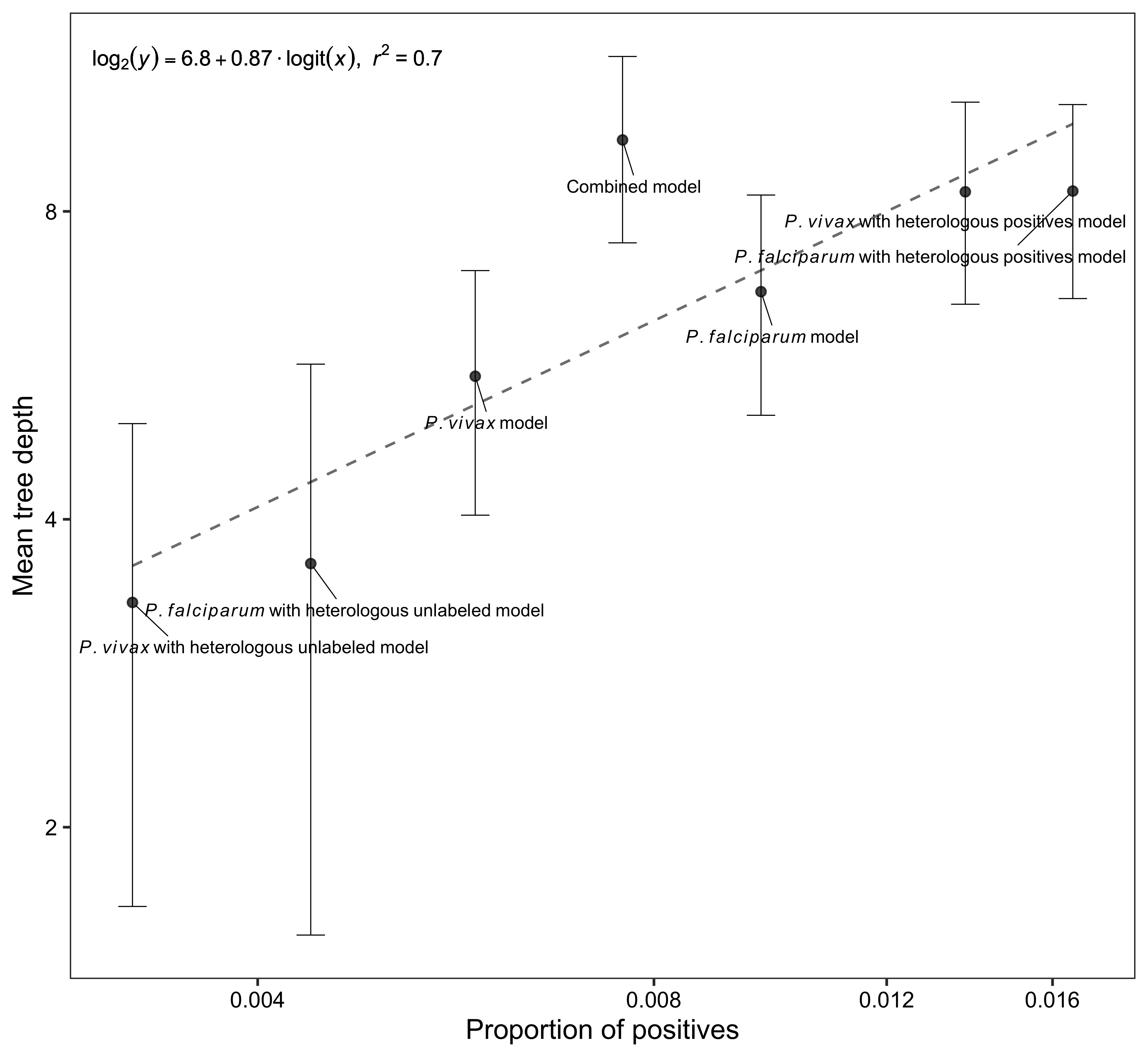

sessionInfo()

## R version 4.2.3 (2023-03-15)
## Platform: x86_64-apple-darwin17.0 (64-bit)
## Running under: macOS Big Sur ... 10.16
## 
## Matrix products: default
## BLAS:   /Library/Frameworks/R.framework/Versions/4.2/Resources/lib/libRblas.0.dylib
## LAPACK: /Library/Frameworks/R.framework/Versions/4.2/Resources/lib/libRlapack.dylib
## 
## locale:
## [1] en_US.UTF-8/en_US.UTF-8/en_US.UTF-8/C/en_US.UTF-8/en_US.UTF-8
## 
## attached base packages:
## [1] stats     graphics  grDevices utils     datasets  methods   base     
## 
## other attached packages:
##  [1] ggrepel_0.9.3     psych_2.3.3       reticulate_1.28   DT_0.27          
##  [5] rcompanion_2.4.30 rlist_0.4.6.2     scales_1.2.1      ggsci_3.0.0      
##  [9] pracma_2.4.2      cowplot_1.1.1     gghalves_0.1.4    ggdist_3.2.1     
## [13] reshape2_1.4.4    ggplot2_3.4.2    
## 
## loaded via a namespace (and not attached):
##  [1] nlme_3.1-162         matrixStats_0.63.0   httr_1.4.6          
##  [4] rprojroot_2.0.3      R.cache_0.16.0       tools_4.2.3         
##  [7] bslib_0.4.2          utf8_1.2.3           R6_2.5.1            
## [10] nortest_1.0-4        colorspace_2.1-0     withr_2.5.0         
## [13] mnormt_2.1.1         tidyselect_1.2.0     Exact_3.2           
## [16] compiler_4.2.3       cli_3.6.1            expm_0.999-7        
## [19] sandwich_3.0-2       bookdown_0.34        sass_0.4.6          
## [22] lmtest_0.9-40        mvtnorm_1.1-3        proxy_0.4-27        
## [25] multcompView_0.1-9   stringr_1.5.0        digest_0.6.31       
## [28] rmarkdown_2.21       R.utils_2.12.2       pkgconfig_2.0.3     
## [31] htmltools_0.5.5      styler_1.9.1         fastmap_1.1.1       
## [34] highr_0.10           htmlwidgets_1.6.2    rlang_1.1.1         
## [37] readxl_1.4.2         rstudioapi_0.14      jquerylib_0.1.4     
## [40] farver_2.1.1         generics_0.1.3       zoo_1.8-12          
## [43] jsonlite_1.8.4       crosstalk_1.2.0      dplyr_1.1.2         
## [46] R.oo_1.25.0          distributional_0.3.2 magrittr_2.0.3      
## [49] modeltools_0.2-23    Matrix_1.5-4         Rcpp_1.0.10         
## [52] DescTools_0.99.48    munsell_0.5.0        fansi_1.0.4         
## [55] lifecycle_1.0.3      R.methodsS3_1.8.2    stringi_1.7.12      
## [58] multcomp_1.4-23      yaml_2.3.7           MASS_7.3-60         
## [61] rootSolve_1.8.2.3    plyr_1.8.8           grid_4.2.3          
## [64] parallel_4.2.3       lmom_2.9             lattice_0.21-8      
## [67] splines_4.2.3        knitr_1.42           pillar_1.9.0        
## [70] boot_1.3-28.1        gld_2.6.6            codetools_0.2-19    
## [73] stats4_4.2.3         glue_1.6.2           evaluate_0.21       
## [76] data.table_1.14.8    vctrs_0.6.2          png_0.1-8           
## [79] cellranger_1.1.0     gtable_0.3.3         purrr_1.0.1         
## [82] cachem_1.0.8         xfun_0.39            coin_1.4-2          
## [85] libcoin_1.0-9        e1071_1.7-13         class_7.3-22        
## [88] survival_3.5-5       tibble_3.2.1         TH.data_1.1-2       
## [91] ellipsis_0.3.2       here_1.0.1

session_info.show()

## -----
## numpy               1.19.0
## pandas              1.3.2
## purf                NA
## session_info        1.0.0
## -----
## Python 3.8.2 (default, Mar 26 2020, 10:45:18) [Clang 4.0.1 (tags/RELEASE_401/final)]
## macOS-10.16-x86_64-i386-64bit
## -----
## Session information updated at 2023-05-18 12:35