Section 5 Model interpretation

5.1 Proximity matrix calculation

5.1.1 Analysis

In Python:

library(reticulate)
use_condaenv("/Users/renee/Library/r-miniconda/envs/purf/bin/python")

import pandas as pd
import numpy as np
import pickle
from purf.pu_ensemble import PURandomForestClassifier
from sklearn.impute import SimpleImputer
from sklearn.ensemble._forest import _generate_unsampled_indices
import multiprocessing
from joblib import Parallel, delayed
num_cores = multiprocessing.cpu_count()
import session_info

5.1.1.1 Pv data set

data = pd.read_csv('./other_data/pv_ml_input.csv', index_col=0)
features = data.iloc[:, 1:]
outcome = np.array(data.antigen_label)

# Imputation
imputer = SimpleImputer(strategy='median')
X = imputer.fit_transform(features)

# Load model
model_tree_filtered = pickle.load(open('./pickle_data/pv_0.5_purf_tree_filtering.pkl', 'rb'))
model = model_tree_filtered['model']
weights = model_tree_filtered['weights']

def calculate_proximity_(trees, y, leaf_indices):
    same_leaf_mat = np.zeros([y.shape[0], y.shape[0]])
    same_oob_mat = np.zeros([y.shape[0], y.shape[0]])
    for idx, tree in enumerate(trees):
        oob_indices = _generate_unsampled_indices(tree.random_state, y.shape[0], y.shape[0])
        for i in oob_indices:
            for j in oob_indices:
                same_oob_mat[i, j] += 1
                if leaf_indices[i, idx] == leaf_indices[j, idx]:
                    same_leaf_mat[i, j] += 1
    return (same_leaf_mat, same_oob_mat)

trees = model.estimators_
leaf_indices = model.apply(X)
idx_list = [i for i in range(len(trees)) if weights[i] == 1]
idx_list = np.array_split(idx_list, 1000)

res = Parallel(n_jobs=num_cores)(
    delayed(calculate_proximity_)(list(trees[i] for i in idx), outcome, leaf_indices[:, idx]) for idx in idx_list)

same_leaf_mat = sum([r[0] for r in res])
same_oob_mat = sum([r[1] for r in res])

prox_mat = pd.DataFrame(np.divide(same_leaf_mat, same_oob_mat, out=np.zeros_like(same_leaf_mat), 
                        where=same_oob_mat!=0))
prox_mat.index = features.index
prox_mat.columns = features.index
prox_mat.to_csv('~/Downloads/pv_proximity_values.csv', index=False)

5.1.1.2 Pv + Pf combined data set

data = pd.read_csv('./data/supplementary_data_4_pfpv_ml_input.csv', index_col=0)
features = data.iloc[:, 1:]
outcome = np.array(data.antigen_label)

# Imputation
imputer = SimpleImputer(strategy='median')
X = imputer.fit_transform(features)

# Load model
model_tree_filtered = pickle.load(open('./pickle_data/pfpv_0.5_purf_tree_filtering.pkl', 'rb'))
model = model_tree_filtered['model']
weights = model_tree_filtered['weights']

def calculate_proximity_(trees, y, leaf_indices):
    same_leaf_mat = np.zeros([y.shape[0], y.shape[0]])
    same_oob_mat = np.zeros([y.shape[0], y.shape[0]])
    for idx, tree in enumerate(trees):
        oob_indices = _generate_unsampled_indices(tree.random_state, y.shape[0], y.shape[0])
        for i in oob_indices:
            for j in oob_indices:
                same_oob_mat[i, j] += 1
                if leaf_indices[i, idx] == leaf_indices[j, idx]:
                    same_leaf_mat[i, j] += 1
    return (same_leaf_mat, same_oob_mat)

trees = model.estimators_
leaf_indices = model.apply(X)
idx_list = [i for i in range(len(trees)) if weights[i] == 1]
idx_list = np.array_split(idx_list, 1000)

res = Parallel(n_jobs=num_cores)(
    delayed(calculate_proximity_)(list(trees[i] for i in idx), outcome, leaf_indices[:, idx]) for idx in idx_list)

same_leaf_mat = sum([r[0] for r in res])
same_oob_mat = sum([r[1] for r in res])

prox_mat = pd.DataFrame(np.divide(same_leaf_mat, same_oob_mat, out=np.zeros_like(same_leaf_mat), 
                        where=same_oob_mat!=0))
prox_mat.index = features.index
prox_mat.columns = features.index
prox_mat.to_csv('~/Downloads/pfpv_proximity_values.csv', index=False)

In R:

# Multidimensional scaling
prox_mat <- read.csv("~/Downloads/pv_proximity_values.csv", check.names = FALSE)
mds <- cmdscale(as.dist(1 - prox_mat), k = ncol(prox_mat) - 1, eig = TRUE)
var_explained <- round(mds$eig * 100 / sum(mds$eig), 2)
print(paste0("Dimension 1 (", var_explained[1], "%)")) # 41.44%
print(paste0("Dimension 2 (", var_explained[2], "%)")) # 8.64%
print(paste0("Dimension 3 (", var_explained[3], "%)")) # 4.72%

mds <- as.data.frame(mds$points)
write.csv(mds, "~/Downloads/mds_pv_proximity_values.csv")

prox_mat <- read.csv("~/Downloads/pfpv_proximity_values.csv", check.names = FALSE)
mds <- cmdscale(as.dist(1 - prox_mat), k = ncol(prox_mat) - 1, eig = TRUE)
var_explained <- round(mds$eig * 100 / sum(mds$eig), 2)
print(paste0("Dimension 1 (", var_explained[1], "%)")) # 37.91%
print(paste0("Dimension 2 (", var_explained[2], "%)")) # 7.88%
print(paste0("Dimension 3 (", var_explained[3], "%)")) # 4.79%

mds <- as.data.frame(mds$points)
write.csv(mds, "~/Downloads/mds_pfpv_proximity_values.csv")

5.1.2 Plotting

In R:

library(umap)
library(ggplot2)
library(ggrepel)
library(cowplot)

5.1.2.1 Pv + Pf combined data set

data <- read.csv("~/Downloads/mds_pfpv_proximity_values.csv", row.names = 1, check.names = FALSE)

set.seed(22)
umap_res <- umap(data)
umap_df <- data.frame(umap_res$layout)
save(umap_df, file = "./rdata/pfpv_prox_mds_umap.RData")

data <- read.csv("./data/supplementary_data_5_pfpv_purf_oob_predictions.csv", row.names = 1, check.names = FALSE)[5394:11884, ]
load("./rdata/pfpv_prox_mds_umap.RData")
umap_df_ <- umap_df[1:5393, ]
umap_df <- umap_df[5394:11884, ]
umap_df$label <- data$antigen_label
umap_df$score <- data$`OOB score filtered`
umap_df_text <- umap_df[umap_df$label == 1, ]
umap_df_text$label_text <- ""
umap_df_text$label_text[rownames(umap_df_text) == "PVP01_0835600.1-p1"] <- "CSP"
umap_df_text$label_text[rownames(umap_df_text) == "PVP01_0623800.1-p1"] <- "DBP"
umap_df_text$label_text[rownames(umap_df_text) == "PVP01_0728900.1-p1"] <- "MSP1"

umap_p1 <- ggplot() +
  geom_point(data = umap_df_, aes(x = X1, y = X2), color = "grey90", alpha = 0.5) +
  geom_point(data = umap_df[umap_df$label == 0, ], aes(x = X1, y = X2, color = score), alpha = 0.5) +
  geom_point(
    data = umap_df[umap_df$label == 1, ], aes(x = X1, y = X2, shape = factor(21)), color = "black",
    fill = "#FCB40A", stroke = 0.3, size = 2, alpha = 0.9
  ) +
  geom_text_repel(
    data = umap_df_text, aes(x = X1, y = X2, label = label_text), size = 3.5,
    nudge_x = 1, nudge_y = -1, point.padding = 0.1
  ) +
  scale_color_gradient2(low = "#3399FF", mid = "white", high = "#FF3399", midpoint = 0.5, limits = c(0, 1)) +
  scale_shape_manual(values = c(21), labels = c("Known antigens")) +
  theme_bw() +
  theme(
    panel.grid.major = element_blank(),
    panel.grid.minor = element_blank(),
    plot.margin = ggplot2::margin(5, 5, 5, 5, "pt"),
    axis.title = element_text(colour = "black"),
    axis.text = element_text(colour = "black"),
    legend.position = "none"
  ) +
  xlab("Dimension 1") +
  ylab("Dimension 2")

data <- read.csv("./data/supplementary_data_5_pfpv_purf_oob_predictions.csv", row.names = 1, check.names = FALSE)[1:5393, ]
load("./rdata/pfpv_prox_mds_umap.RData")
umap_df_ <- umap_df[5394:11884, ]
umap_df <- umap_df[1:5393, ]
umap_df$label <- data$antigen_label
umap_df$score <- data$`OOB score filtered`
umap_df_text <- umap_df[umap_df$label == 1, ]
umap_df_text$label_text <- ""
umap_df_text$label_text[rownames(umap_df_text) == "PF3D7_0304600.1-p1"] <- "CSP"
umap_df_text$label_text[rownames(umap_df_text) == "PF3D7_0424100.1-p1"] <- "RH5"
umap_df_text$label_text[rownames(umap_df_text) == "PF3D7_0206900.1-p1"] <- "MSP5"
umap_df_text$label_text[rownames(umap_df_text) == "PF3D7_0209000.1-p1"] <- "P230"

umap_p2 <- ggplot() +
  geom_point(data = umap_df_, aes(x = X1, y = X2), color = "grey90", alpha = 0.5) +
  geom_point(data = umap_df[umap_df$label == 0, ], aes(x = X1, y = X2, color = score), alpha = 0.5) +
  geom_point(
    data = umap_df[umap_df$label == 1, ], aes(x = X1, y = X2), shape = 21, color = "black",
    fill = "#FCB40A", stroke = 0.3, size = 2, alpha = 0.9
  ) +
  geom_text_repel(
    data = umap_df_text, aes(x = X1, y = X2, label = label_text), size = 3.5,
    nudge_x = 1.5, nudge_y = -1, point.padding = 0.1
  ) +
  scale_color_gradient2(low = "#3399FF", mid = "white", high = "#FF3399", midpoint = 0.5, limits = c(0, 1)) +
  theme_bw() +
  theme(
    panel.grid.major = element_blank(),
    panel.grid.minor = element_blank(),
    plot.margin = ggplot2::margin(5, 5, 5, 5, "pt"),
    axis.title = element_text(colour = "black"),
    axis.text = element_text(colour = "black"),
    legend.position = "none"
  ) +
  xlab("Dimension 1") +
  ylab("Dimension 2")

legend <- get_legend(umap_p2 +
  theme(
    legend.direction = "horizontal",
    legend.position = "bottom",
    legend.title = element_text(vjust = 0.8, colour = "black")
  ) +
  guides(
    color = guide_colorbar(title = "Score"),
    shape = guide_legend(title = "")
  ))

umap_p_combined <- plot_grid(umap_p1, umap_p2,
  plot_grid(NULL, legend, rel_widths = c(0.15, 0.85)),
  ncol = 2,
  rel_heights = c(1, 0.2), labels = c("a", "b", "", "")
)
umap_p_combined

png(file = "./figures/Fig 3.png", width = 6000, height = 3500, res = 600)
print(umap_p_combined)
dev.off()

pdf(file = "../figures/Fig 3.pdf", width = 12, height = 7)
print(umap_p_combined)
dev.off()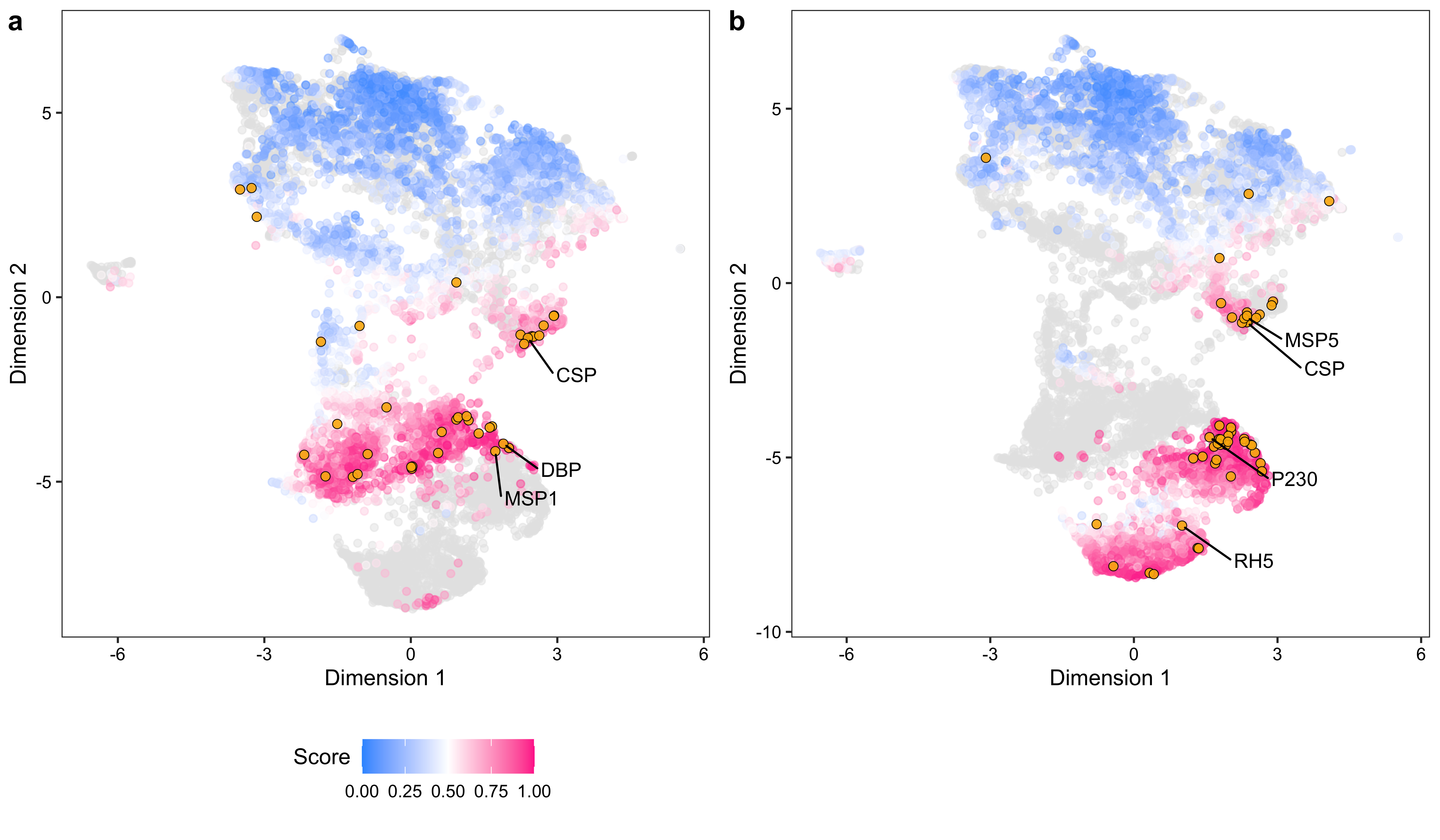

5.2 Clustering of predicted positives

5.2.1 Analysis

In R:

library(DT)
library(factoextra)
library(NbClust)
library(cluster)
library(dendextend)
library(umap)
library(ggplot2)
library(ggrepel)
library(cowplot)
library(scales)
library(rcompanion)

scientific <- function(x) {
  ifelse(x == 0, "0", gsub("e", " * 10^", scientific_format(digits = 3)(x)))
}

calculate_association <- function(clusters) {
  species <- sapply(names(clusters), function(x) if (startsWith(x, "PF3D7")) "pf" else "pv")
  M <- table(clusters, species)
  Xsq <- chisq.test(M, correct = FALSE)
  cramerV <- cramerV(M, ci = TRUE)
  return(list(
    M = M, xsq_pval = scientific(as.numeric(Xsq$p.value)),
    cramerV = sprintf("%0.2f", cramerV)
  ))
}

pfpv_data <- read.csv("./data/supplementary_data_5_pfpv_purf_oob_predictions.csv", row.names = 1, check.names = FALSE)
pred_pos <- rownames(pfpv_data)[pfpv_data$`OOB score filtered` >= 0.5]
pfpv_prox <- read.csv("~/Downloads/pfpv_proximity_values.csv", check.names = FALSE)
pred_pos_dist <- 1 - pfpv_prox
rownames(pred_pos_dist) <- colnames(pred_pos_dist)
pred_pos_dist <- pred_pos_dist[rownames(pred_pos_dist) %in% pred_pos, colnames(pred_pos_dist) %in% pred_pos]

pred_pos_hc <- hclust(as.dist(pred_pos_dist), method = "ward.D2")
save(pred_pos_hc, file = "./rdata/pred_pos_clusters.RData")

load(file = "./rdata/pred_pos_clusters.RData")
clusters <- cutree(pred_pos_hc, k = 2)
calculate_association(clusters)

## $M
##         species
## clusters   pf   pv
##        1 1695 1918
##        2  979  759
## 
## $xsq_pval
## [1] "1.11 * 10^-10"
## 
## $cramerV
## [1] "0.09" "0.06" "0.11"

data <- read.csv("./data/supplementary_data_5_pfpv_purf_oob_predictions.csv", row.names = 1, check.names = FALSE)
load("./rdata/pfpv_prox_mds_umap.RData")
umap_df$label <- data$antigen_label
umap_df_ <- umap_df[!rownames(umap_df) %in% names(clusters), ]
umap_df <- rbind(umap_df[umap_df$label == 1, ], umap_df[rownames(umap_df) %in% names(clusters), ])
umap_df$group <- ""
umap_df$group[umap_df$label == 1] <- "Known antigen"
umap_df$group[rownames(umap_df) %in% c("PF3D7_0304600.1-p1", "PF3D7_0424100.1-p1", "PF3D7_0206900.1-p1", "PF3D7_0209000.1-p1", "PVP01_0835600.1-p1", "PVP01_0623800.1-p1", "PVP01_0728900.1-p1")] <- "Reference antigen"
umap_df$group[rownames(umap_df) %in% names(clusters)[clusters == 1]] <- "Group 1"
umap_df$group[rownames(umap_df) %in% names(clusters)[clusters == 2]] <- "Group 2"
umap_df_text <- umap_df[umap_df$label == 1, ]
umap_df_text$label_text <- ""
umap_df_text$label_text[rownames(umap_df_text) == "PF3D7_0304600.1-p1"] <- "PfCSP"
umap_df_text$label_text[rownames(umap_df_text) == "PF3D7_0424100.1-p1"] <- "RH5"
umap_df_text$label_text[rownames(umap_df_text) == "PF3D7_0206900.1-p1"] <- "MSP5"
umap_df_text$label_text[rownames(umap_df_text) == "PF3D7_0209000.1-p1"] <- "P230"
umap_df_text$label_text[rownames(umap_df_text) == "PVP01_0835600.1-p1"] <- "PvCSP"
umap_df_text$label_text[rownames(umap_df_text) == "PVP01_0623800.1-p1"] <- "DBP"
umap_df_text$label_text[rownames(umap_df_text) == "PVP01_0728900.1-p1"] <- "MSP1"

umap_p1 <- ggplot() +
  geom_point(data = umap_df_, aes(x = X1, y = X2), color = "grey90", alpha = 0.5) +
  geom_point(data = umap_df[umap_df$label == 0, ], aes(x = X1, y = X2, fill = group), shape = 21, alpha = 0.5) +
  scale_fill_manual(
    breaks = c("Group 1", "Group 2"), values = c("#A552FD", "#FD529B"),
    labels = c("Predicted antigen (Group 1)", "Predicted antigen (Group 2)")
  ) +
  geom_point(
    data = umap_df[umap_df$label == 1, ], aes(x = X1, y = X2), shape = 21, color = "black",
    fill = "#FFFF33", stroke = 0.3, size = 2, alpha = 0.5
  ) +
  geom_text_repel(
    data = umap_df_text, aes(x = X1, y = X2, label = label_text), size = 3.5,
    nudge_x = 1.5, nudge_y = -1, point.padding = 0.1
  ) +
  theme_bw() +
  theme(
    panel.grid.major = element_blank(),
    panel.grid.minor = element_blank(),
    plot.margin = ggplot2::margin(5, 5, 5, 5, "pt"),
    axis.title = element_text(colour = "black"),
    axis.text = element_text(colour = "black"),
    legend.position = "bottom"
  ) +
  guides(fill = guide_legend(title = "")) +
  xlab("Dimension 1") +
  ylab("Dimension 2")

load(file = "./rdata/pred_pos_clusters.RData")
pred_pos_hc_list <- get_subdendrograms(as.dendrogram(pred_pos_hc), 2)
pred_pos_hc_list_2 <- get_subdendrograms(as.dendrogram(pred_pos_hc_list[[1]]), 2)
clusters <- c(
  rep(1, nleaves(pred_pos_hc_list_2[[1]])),
  rep(2, nleaves(pred_pos_hc_list_2[[2]]))
)
names(clusters) <- c(labels(pred_pos_hc_list_2[[1]]), labels(pred_pos_hc_list_2[[2]]))
save(pred_pos_hc, pred_pos_hc_list, pred_pos_hc_list_2,
  file = "./rdata/pred_pos_clusters.RData"
)

load(file = "./rdata/pred_pos_clusters.RData")
clusters <- c(
  rep(1, nleaves(pred_pos_hc_list_2[[1]])),
  rep(2, nleaves(pred_pos_hc_list_2[[2]]))
)
names(clusters) <- c(labels(pred_pos_hc_list_2[[1]]), labels(pred_pos_hc_list_2[[2]]))
calculate_association(clusters)

## $M
##         species
## clusters   pf   pv
##        1  147  519
##        2 1548 1399
## 
## $xsq_pval
## [1] "6.5 * 10^-46"
## 
## $cramerV
## [1] "0.24" "0.21" "0.27"

data <- read.csv("./data/supplementary_data_5_pfpv_purf_oob_predictions.csv", row.names = 1, check.names = FALSE)
load("./rdata/pfpv_prox_mds_umap.RData")
umap_df$label <- data$antigen_label
umap_df_ <- umap_df[!rownames(umap_df) %in% names(clusters), ]
umap_df <- rbind(umap_df[umap_df$label == 1, ], umap_df[rownames(umap_df) %in% names(clusters), ])
umap_df$group <- ""
umap_df$group[umap_df$label == 1] <- "Known antigen"
umap_df$group[rownames(umap_df) %in% c("PF3D7_0304600.1-p1", "PF3D7_0424100.1-p1", "PF3D7_0206900.1-p1", "PF3D7_0209000.1-p1", "PVP01_0835600.1-p1", "PVP01_0623800.1-p1", "PVP01_0728900.1-p1")] <- "Reference antigen"
umap_df$group[rownames(umap_df) %in% names(clusters)[clusters == 1]] <- "Group 1"
umap_df$group[rownames(umap_df) %in% names(clusters)[clusters == 2]] <- "Group 2"
umap_df_text <- umap_df[umap_df$label == 1, ]
umap_df_text$label_text <- ""
umap_df_text$label_text[rownames(umap_df_text) == "PF3D7_0304600.1-p1"] <- "PfCSP"
umap_df_text$label_text[rownames(umap_df_text) == "PF3D7_0424100.1-p1"] <- "RH5"
umap_df_text$label_text[rownames(umap_df_text) == "PF3D7_0206900.1-p1"] <- "MSP5"
umap_df_text$label_text[rownames(umap_df_text) == "PF3D7_0209000.1-p1"] <- "P230"
umap_df_text$label_text[rownames(umap_df_text) == "PVP01_0835600.1-p1"] <- "PvCSP"
umap_df_text$label_text[rownames(umap_df_text) == "PVP01_0623800.1-p1"] <- "DBP"
umap_df_text$label_text[rownames(umap_df_text) == "PVP01_0728900.1-p1"] <- "MSP1"

umap_p2 <- ggplot() +
  geom_point(data = umap_df_, aes(x = X1, y = X2), color = "grey90", alpha = 0.5) +
  geom_point(data = umap_df[umap_df$label == 0, ], aes(x = X1, y = X2, fill = group), shape = 21, alpha = 0.5) +
  scale_fill_manual(
    breaks = c("Group 1", "Group 2"), values = c("#A552FD", "#53F4EF"),
    labels = c("Predicted antigen (Group 1)", "Predicted antigen (Group 2)")
  ) +
  geom_point(
    data = umap_df[umap_df$label == 1, ], aes(x = X1, y = X2), shape = 21, color = "black",
    fill = "#FFFF33", stroke = 0.3, size = 2, alpha = 0.5
  ) +
  geom_text_repel(
    data = umap_df_text, aes(x = X1, y = X2, label = label_text), size = 3.5,
    nudge_x = 1.5, nudge_y = -1, point.padding = 0.1
  ) +
  theme_bw() +
  theme(
    panel.grid.major = element_blank(),
    panel.grid.minor = element_blank(),
    plot.margin = ggplot2::margin(5, 5, 5, 5, "pt"),
    axis.title = element_text(colour = "black"),
    axis.text = element_text(colour = "black"),
    legend.position = "bottom"
  ) +
  guides(fill = guide_legend(title = "")) +
  xlab("Dimension 1") +
  ylab("Dimension 2")

load(file = "./rdata/pred_pos_clusters.RData")
pred_pos_hc_list_3 <- get_subdendrograms(as.dendrogram(pred_pos_hc_list_2[[2]]), 2)
clusters <- c(
  rep(1, nleaves(pred_pos_hc_list_3[[1]])),
  rep(2, nleaves(pred_pos_hc_list_3[[2]]))
)
names(clusters) <- c(labels(pred_pos_hc_list_3[[1]]), labels(pred_pos_hc_list_3[[2]]))
save(pred_pos_hc, pred_pos_hc_list, pred_pos_hc_list_2, pred_pos_hc_list_3,
  file = "./rdata/pred_pos_clusters.RData"
)

load(file = "./rdata/pred_pos_clusters.RData")
clusters <- c(
  rep(1, nleaves(pred_pos_hc_list_3[[1]])),
  rep(2, nleaves(pred_pos_hc_list_3[[2]]))
)
names(clusters) <- c(labels(pred_pos_hc_list_3[[1]]), labels(pred_pos_hc_list_3[[2]]))
calculate_association(clusters)

## $M
##         species
## clusters   pf   pv
##        1 1505   40
##        2   43 1359
## 
## $xsq_pval
## [1] "0"
## 
## $cramerV
## [1] "0.94" "0.93" "0.95"

data <- read.csv("./data/supplementary_data_5_pfpv_purf_oob_predictions.csv", row.names = 1, check.names = FALSE)
load("./rdata/pfpv_prox_mds_umap.RData")
umap_df$label <- data$antigen_label
umap_df_ <- umap_df[!rownames(umap_df) %in% names(clusters), ]
umap_df <- rbind(umap_df[umap_df$label == 1, ], umap_df[rownames(umap_df) %in% names(clusters), ])
umap_df$group <- ""
umap_df$group[umap_df$label == 1] <- "Known antigen"
umap_df$group[rownames(umap_df) %in% c("PF3D7_0304600.1-p1", "PF3D7_0424100.1-p1", "PF3D7_0206900.1-p1", "PF3D7_0209000.1-p1", "PVP01_0835600.1-p1", "PVP01_0623800.1-p1", "PVP01_0728900.1-p1")] <- "Reference antigen"
umap_df$group[rownames(umap_df) %in% names(clusters)[clusters == 1]] <- "Group 1"
umap_df$group[rownames(umap_df) %in% names(clusters)[clusters == 2]] <- "Group 2"
umap_df_text <- umap_df[umap_df$label == 1, ]
umap_df_text$label_text <- ""
umap_df_text$label_text[rownames(umap_df_text) == "PF3D7_0304600.1-p1"] <- "PfCSP"
umap_df_text$label_text[rownames(umap_df_text) == "PF3D7_0424100.1-p1"] <- "RH5"
umap_df_text$label_text[rownames(umap_df_text) == "PF3D7_0206900.1-p1"] <- "MSP5"
umap_df_text$label_text[rownames(umap_df_text) == "PF3D7_0209000.1-p1"] <- "P230"
umap_df_text$label_text[rownames(umap_df_text) == "PVP01_0835600.1-p1"] <- "PvCSP"
umap_df_text$label_text[rownames(umap_df_text) == "PVP01_0623800.1-p1"] <- "DBP"
umap_df_text$label_text[rownames(umap_df_text) == "PVP01_0728900.1-p1"] <- "MSP1"

umap_p3 <- ggplot() +
  geom_point(data = umap_df_, aes(x = X1, y = X2), color = "grey90", alpha = 0.5) +
  geom_point(data = umap_df[umap_df$label == 0, ], aes(x = X1, y = X2, fill = group), shape = 21, alpha = 0.5) +
  scale_fill_manual(
    breaks = c("Group 1", "Group 2"), values = c("#F49553", "#53F4EF"),
    labels = c("Predicted antigen (Group 1)", "Predicted antigen (Group 2)")
  ) +
  geom_point(
    data = umap_df[umap_df$label == 1, ], aes(x = X1, y = X2), shape = 21, color = "black",
    fill = "#FFFF33", stroke = 0.3, size = 2, alpha = 0.5
  ) +
  geom_text_repel(
    data = umap_df_text, aes(x = X1, y = X2, label = label_text), size = 3.5,
    nudge_x = 1.5, nudge_y = -1, point.padding = 0.1
  ) +
  theme_bw() +
  theme(
    panel.grid.major = element_blank(),
    panel.grid.minor = element_blank(),
    plot.margin = ggplot2::margin(5, 5, 5, 5, "pt"),
    axis.title = element_text(colour = "black"),
    axis.text = element_text(colour = "black"),
    legend.position = "bottom"
  ) +
  guides(fill = guide_legend(title = "")) +
  xlab("Dimension 1") +
  ylab("Dimension 2")

load(file = "./rdata/pred_pos_clusters.RData")
pred_pos_hc_list_4 <- get_subdendrograms(as.dendrogram(pred_pos_hc_list_3[[1]]), 2)
clusters <- c(
  rep(1, nleaves(pred_pos_hc_list_4[[1]])),
  rep(2, nleaves(pred_pos_hc_list_4[[2]]))
)
names(clusters) <- c(labels(pred_pos_hc_list_4[[1]]), labels(pred_pos_hc_list_4[[2]]))
save(pred_pos_hc, pred_pos_hc_list, pred_pos_hc_list_2, pred_pos_hc_list_3, pred_pos_hc_list_4,
  file = "./rdata/pred_pos_clusters.RData"
)

load(file = "./rdata/pred_pos_clusters.RData")
clusters <- c(
  rep(1, nleaves(pred_pos_hc_list_4[[1]])),
  rep(2, nleaves(pred_pos_hc_list_4[[2]]))
)
names(clusters) <- c(labels(pred_pos_hc_list_4[[1]]), labels(pred_pos_hc_list_4[[2]]))
calculate_association(clusters)

## $M
##         species
## clusters  pf  pv
##        1 563  18
##        2 942  22
## 
## $xsq_pval
## [1] "3.28 * 10^-01"
## 
## $cramerV
## [1] "0.02" "0.00" "0.08"

data <- read.csv("./data/supplementary_data_5_pfpv_purf_oob_predictions.csv", row.names = 1, check.names = FALSE)
load("./rdata/pfpv_prox_mds_umap.RData")
umap_df$label <- data$antigen_label
umap_df_ <- umap_df[!rownames(umap_df) %in% names(clusters), ]
umap_df <- rbind(umap_df[umap_df$label == 1, ], umap_df[rownames(umap_df) %in% names(clusters), ])
umap_df$group <- ""
umap_df$group[umap_df$label == 1] <- "Known antigen"
umap_df$group[rownames(umap_df) %in% c("PF3D7_0304600.1-p1", "PF3D7_0424100.1-p1", "PF3D7_0206900.1-p1", "PF3D7_0209000.1-p1", "PVP01_0835600.1-p1", "PVP01_0623800.1-p1", "PVP01_0728900.1-p1")] <- "Reference antigen"
umap_df$group[rownames(umap_df) %in% names(clusters)[clusters == 1]] <- "Group 1"
umap_df$group[rownames(umap_df) %in% names(clusters)[clusters == 2]] <- "Group 2"
umap_df_text <- umap_df[umap_df$label == 1, ]
umap_df_text$label_text <- ""
umap_df_text$label_text[rownames(umap_df_text) == "PF3D7_0304600.1-p1"] <- "PfCSP"
umap_df_text$label_text[rownames(umap_df_text) == "PF3D7_0424100.1-p1"] <- "RH5"
umap_df_text$label_text[rownames(umap_df_text) == "PF3D7_0206900.1-p1"] <- "MSP5"
umap_df_text$label_text[rownames(umap_df_text) == "PF3D7_0209000.1-p1"] <- "P230"
umap_df_text$label_text[rownames(umap_df_text) == "PVP01_0835600.1-p1"] <- "PvCSP"
umap_df_text$label_text[rownames(umap_df_text) == "PVP01_0623800.1-p1"] <- "DBP"
umap_df_text$label_text[rownames(umap_df_text) == "PVP01_0728900.1-p1"] <- "MSP1"

umap_p4 <- ggplot() +
  geom_point(data = umap_df_, aes(x = X1, y = X2), color = "grey90", alpha = 0.5) +
  geom_point(data = umap_df[umap_df$label == 0, ], aes(x = X1, y = X2, fill = group), shape = 21, alpha = 0.5) +
  scale_fill_manual(
    breaks = c("Group 1", "Group 2"), values = c("#F49553", "#D953F4"),
    labels = c("Predicted antigen (Group 1)", "Predicted antigen (Group 2)")
  ) +
  geom_point(
    data = umap_df[umap_df$label == 1, ], aes(x = X1, y = X2), shape = 21, color = "black",
    fill = "#FFFF33", stroke = 0.3, size = 2, alpha = 0.5
  ) +
  geom_text_repel(
    data = umap_df_text, aes(x = X1, y = X2, label = label_text), size = 3.5,
    nudge_x = 1.5, nudge_y = -1, point.padding = 0.1
  ) +
  theme_bw() +
  theme(
    panel.grid.major = element_blank(),
    panel.grid.minor = element_blank(),
    plot.margin = ggplot2::margin(5, 5, 5, 5, "pt"),
    axis.title = element_text(colour = "black"),
    axis.text = element_text(colour = "black"),
    legend.position = "bottom"
  ) +
  guides(fill = guide_legend(title = "")) +
  xlab("Dimension 1") +
  ylab("Dimension 2")

umap_p_combined <- plot_grid(umap_p1, umap_p2, umap_p3, umap_p4,
  nrow = 2,
  labels = c("a", "b", "c", "d")
)
umap_p_combined

png(file = "./figures/Supplementary Fig 8.png", width = 6000, height = 6200, res = 600)
print(umap_p_combined)
dev.off()

pdf(file = "../supplementary_figures/Supplementary Fig 8.pdf", width = 12, height = 12.4)
print(umap_p_combined)
dev.off()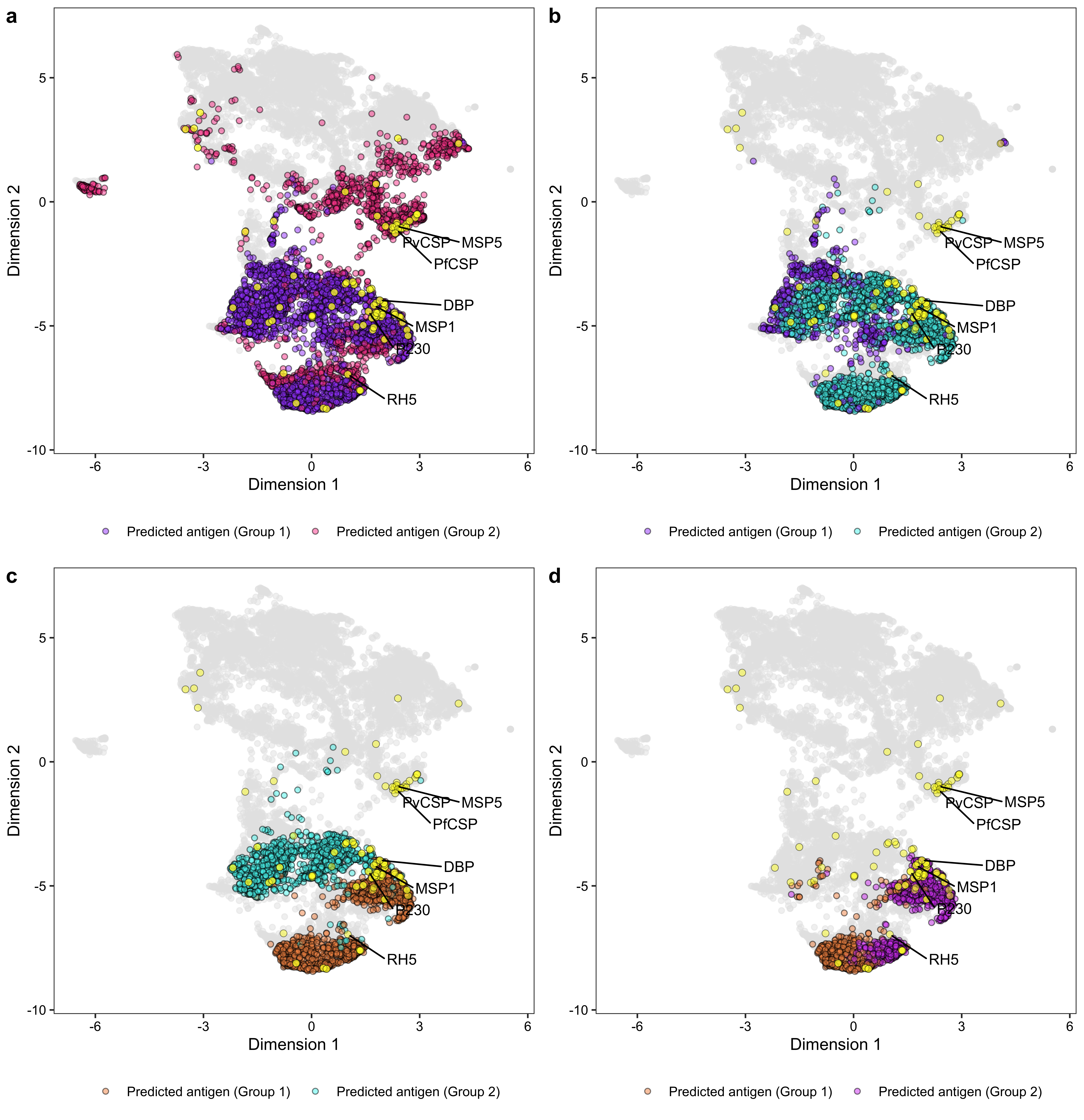

5.3 Comparison of amino acid frequencies between species

5.3.1 Analysis

Python:

library(reticulate)
use_condaenv("/Users/renee/Library/r-miniconda/envs/purf/bin/python")

from Bio import SeqIO
import pandas as pd

ds = pd.read_csv('./data/supplementary_data_5_pfpv_purf_oob_predictions.csv', index_col=0)
pv_records = list(SeqIO.parse('./other_data/combined_PlasmoDB-45_PvivaxP01_AnnotatedProteins_no_pseudo_genes_special_sequences_modified.fasta', 'fasta'))
pf_records = list(SeqIO.parse('./other_data/combined_PlasmoDB-43_Pfalciparum3D7_AnnotatedProteins_no_pseudo_genes_special_sequences_modified.fasta', 'fasta'))

pv_pos = ds[(ds['OOB score filtered'] >= 0.5) & (ds['species'] == 'pv')].index
pf_pos = ds[(ds['OOB score filtered'] >= 0.5) & (ds['species'] == 'pf')].index
pv_neg = ds[(ds['OOB score filtered'] < 0.5) & (ds['species'] == 'pv')].index
pf_neg = ds[(ds['OOB score filtered'] < 0.5) & (ds['species'] == 'pf')].index

pv_pos_records = [record for record in pv_records if record.id in pv_pos]
pf_pos_records = [record for record in pf_records if record.id in pf_pos]
pv_neg_records = [record for record in pv_records if record.id in pv_neg]
pf_neg_records = [record for record in pf_records if record.id in pf_neg]

aa_freq = {}
for i in 'ACDEFGHIKLMNPQRSTVWY':
    aa_freq[i] = [0, 0, 0, 0, 0, 0]
    
for record in pv_records:
    for char in record.seq:
        aa_freq[char][0] += 1

for record in pf_records:
    for char in record.seq:
        aa_freq[char][1] += 1

for record in pv_pos_records:
    for char in record.seq:
        aa_freq[char][2] += 1

for record in pf_pos_records:
    for char in record.seq:
        aa_freq[char][3] += 1

for record in pv_neg_records:
    for char in record.seq:
        aa_freq[char][4] += 1

for record in pf_neg_records:
    for char in record.seq:
        aa_freq[char][5] += 1

res = pd.DataFrame.from_dict(aa_freq)
res.index = ['pv', 'pf', 'pv_pos', 'pf_pos', 'pv_neg', 'pf_neg']
res.to_csv('./other_data/pfpv_aa_freq.csv')

In R:

library(rcompanion)
library(rlist)
library(DT)

scientific <- function(x) {
  ifelse(x == 0, "0", gsub("e", " * 10^", scientific_format(digits = 3)(x)))
}

ds <- read.csv("./other_data/pfpv_aa_freq.csv", row.names = 1)
chisq_pval <- c()
cramer_res <- list()
# Comparison between Pv and Pf
M <- as.table(as.matrix(ds[1:2, ]))
Xsq <- chisq.test(M, correct = FALSE)
cramerV <- cramerV(M, ci = TRUE, R = 100)
chisq_pval <- c(chisq_pval, Xsq$p.value)
cramer_res <- list.append(cramer_res, sprintf("%0.2f", cramerV))
# Comparison between Pv and Pf positives
M <- as.table(as.matrix(ds[3:4, ]))
Xsq <- chisq.test(M, correct = FALSE)
cramerV <- cramerV(M, ci = TRUE, R = 100)
chisq_pval <- c(chisq_pval, Xsq$p.value)
cramer_res <- list.append(cramer_res, sprintf("%0.2f", cramerV))
# Comparison between Pv and Pf negatives
M <- as.table(as.matrix(ds[5:6, ]))
Xsq <- chisq.test(M, correct = FALSE)
cramerV <- cramerV(M, ci = TRUE, R = 100)
chisq_pval <- c(chisq_pval, Xsq$p.value)
cramer_res <- list.append(cramer_res, sprintf("%0.2f", cramerV))
# Save results
df <- as.data.frame(cbind(
  c("Pv vs. Pf", "Pv pos vs. Pf pos", "Pv neg vs. Pf neg"),
  chisq_pval, do.call(rbind, cramer_res)
))
colnames(df) <- c("PURF model", "Chi-squared test p-value", "Cramer's V", "Lower CI", "Upper CI")
df$`Chi-squared test p-value` <- sapply(as.numeric(df$`Chi-squared test p-value`), scientific)
save(df, file = "./rdata/pfpv_aa_freq_comparisons.RData")

load("./rdata/pfpv_aa_freq_comparisons.RData")
df %>%
  datatable(rownames = FALSE)

5.4 Variable importance

5.4.1 Analysis

In Python:

library(reticulate)
use_condaenv("/Users/renee/Library/r-miniconda/envs/purf/bin/python")

import pickle
import pandas as pd
import numpy as np
from sklearn.utils import shuffle
import pickle
from sklearn.impute import SimpleImputer
from sklearn.preprocessing import MinMaxScaler
from scipy.spatial import distance
import multiprocessing
from joblib import Parallel, delayed
num_cores = multiprocessing.cpu_count()
from sklearn.ensemble._forest import _generate_unsampled_indices
import session_info

def calculate_raw_var_imp_(idx, tree, X, y, weight, groups=None):
    rng = np.random.RandomState(idx)
    oob_indices = _generate_unsampled_indices(tree.random_state, y.shape[0], y.shape[0])
    oob_pos = np.intersect1d(oob_indices, np.where(y == 1)[0])
    noutall = len(oob_pos)
    pred = tree.predict_proba(X.iloc[oob_pos,:])[:, 1]
    nrightall = sum(pred == y[oob_pos])
    imprt, impsd = [], []
    if groups is None:
        for var in range(X.shape[1]):
            X_temp = X.copy()
            X_temp.iloc[:, var] = rng.permutation(X_temp.iloc[:, var])
            pred = tree.predict_proba(X_temp.iloc[oob_pos,:])[:, 1]
            nrightimpall = sum(pred == y[oob_pos])
            delta = (nrightall - nrightimpall) / noutall * weight
            imprt.append(delta)
            impsd.append(delta * delta)
    else:
        for grp in np.unique(groups):
            X_temp = X.copy()
            X_temp.iloc[:, groups == grp] = rng.permutation(X_temp.iloc[:, groups == grp])
            pred = tree.predict_proba(X_temp.iloc[oob_pos,:])[:, 1]
            nrightimpall = sum(pred == y[oob_pos])
            delta = (nrightall - nrightimpall) / noutall * weight
            imprt.append(delta)
            impsd.append(delta * delta)
    return (imprt, impsd)
  
def calculate_var_imp(model, features, outcome, num_cores, weights=None, groups=None):
    trees = model.estimators_
    idx_list = [i for i in range(len(trees))]
    if weights is None:
        weights = np.ones(len(trees))
    res = Parallel(n_jobs=num_cores)(
      delayed(calculate_raw_var_imp_)(idx, trees[idx], features, outcome, weights[idx], groups) for idx in idx_list)
    imprt, impsd = [], []
    for i in range(len(idx_list)):
        imprt.append(res[i][0])
        impsd.append(res[i][1])
    imprt = np.array(imprt).sum(axis=0)
    impsd = np.array(impsd).sum(axis=0)
    imprt /= sum(weights)
    impsd = np.sqrt(((impsd / sum(weights)) - imprt * imprt) / sum(weights))
    mda = []
    for i in range(len(imprt)):
        if impsd[i] != 0:
            mda.append(imprt[i] / impsd[i])
        else:
            mda.append(imprt[i])
    if groups is None:
        var_imp = pd.DataFrame({'variable': features.columns, 'meanDecreaseAccuracy': mda})
    else:
        var_imp = pd.DataFrame({'variable': np.unique(groups), 'meanDecreaseAccuracy': mda})
    return var_imp

5.4.1.1 Pv data set

In Python:

data = pd.read_csv('./other_data/pv_ml_input.csv', index_col=0)
features = data.iloc[:, 1:]
outcome = np.array(data.antigen_label)

features, outcome = shuffle(features, outcome, random_state=0)

# Imputation
imputer = SimpleImputer(strategy='median')
X = imputer.fit_transform(features)
X = pd.DataFrame(X, index=features.index, columns=features.columns)
y = outcome
features = X
print('There are %d positives out of %d samples before feature space weighting.' % (sum(y), len(y)))

# Feature space weighting
lab_pos = X.loc[y==1,:]
median = np.median(lab_pos, axis=0)

# Feature space weighting
lab_pos = X.loc[y==1,:]
median = np.median(lab_pos, axis=0)
scaler = MinMaxScaler(feature_range=(1,10))
dist = list()
for i in range(lab_pos.shape[0]):
    dist.append(distance.euclidean(lab_pos.iloc[i, :], median))
    
dist = np.asarray(dist).reshape(-1, 1)
counts = np.round(scaler.fit_transform(dist))
counts = np.array(counts, dtype=np.int64)[:, 0]
X_temp = X.iloc[y==1, :]
X = X.iloc[y==0, :]
y = np.asarray([0] * X.shape[0] + [1] * (sum(counts)))
appended_data = [X]
for i in range(len(counts)):
    appended_data.append(pd.concat([X_temp.iloc[[i]]] * counts[i]))
    
X = pd.concat(appended_data)
print('There are %d positives out of %d samples after feature space weighting.' % (sum(y), len(y)))
features = X
outcome = y
X.to_csv('./other_data/pv_ml_input_processed_weighted.csv')

purf_model = pickle.load(open('./pickle_data/pv_0.5_purf_tree_filtering.pkl', 'rb'))
purf = purf_model['model']
weights = purf_model['weights']

metadata = pd.read_csv('./data/supplementary_data_1_protein_variable_metadata.csv')
groups = metadata.loc[np.isin(metadata['column name'], features.columns), 'category'].array

var_imp = calculate_var_imp(purf, features, outcome, 8, weights)
grp_var_imp = calculate_var_imp(purf, features, outcome, 8, weights, groups)
var_imp.to_csv('./other_data/pv_known_antigen_variable_importance.csv', index=False)
grp_var_imp.to_csv('./other_data/pv_known_antigen_group_variable_importance.csv', index=False)

In R:

prediction <- read.csv("./data/supplementary_data_3_pv_purf_oob_predictions.csv", check.names = FALSE)
known_antigens <- prediction[prediction$antigen_label == 1, ]$protein_id
other_proteins <- prediction[prediction$antigen_label == 0 & prediction$`OOB score filtered` < 0.5, ]$protein_id

set.seed(22)
random_proteins <- sample(other_proteins, size = length(known_antigens), replace = FALSE)

# Load imputed data
data <- read.csv("./other_data/pv_ml_input_processed_weighted.csv")
data <- data[!duplicated(data), ]
compared_group <- sapply(data$protein_id, function(x) if (x %in% known_antigens) 1 else if (x %in% random_proteins) 0 else -1)
data <- data[, 2:ncol(data)]

# Min-max normalization
min_max <- function(x) {
  (x - min(x)) / (max(x) - min(x))
}
data <- data.frame(lapply(data, min_max))

save(compared_group, data, file = "./rdata/pv_known_antigen_wilcox_data.RData")

load(file = "./rdata/pv_known_antigen_wilcox_data.RData")
pval <- c()
for (i in 1:ncol(data)) {
  pval <- c(pval, wilcox.test(data[compared_group == 1, i], data[compared_group == 0, i])$p.value)
}
adj_pval <- p.adjust(pval, method = "BH", n = length(pval))
wilcox_res <- data.frame(variable = colnames(data), adj_pval = adj_pval)
write.csv(wilcox_res, "./other_data/pv_known_antigen_wilcox_res.csv", row.names = FALSE)

5.4.1.2 Pv + Pf combined data set

In Python:

data = pd.read_csv('./data/supplementary_data_4_pfpv_ml_input.csv', index_col=0)
features = data.iloc[:, 1:]
outcome = np.array(data.antigen_label)

features, outcome = shuffle(features, outcome, random_state=0)

# Imputation
imputer = SimpleImputer(strategy='median')
X = imputer.fit_transform(features)
X = pd.DataFrame(X, index=features.index, columns=features.columns)
y = outcome
features = X
print('There are %d positives out of %d samples before feature space weighting.' % (sum(y), len(y)))

# Feature space weighting
lab_pos = X.loc[y==1,:]
median = np.median(lab_pos, axis=0)

# Feature space weighting
lab_pos = X.loc[y==1,:]
median = np.median(lab_pos, axis=0)
scaler = MinMaxScaler(feature_range=(1,10))
dist = list()
for i in range(lab_pos.shape[0]):
    dist.append(distance.euclidean(lab_pos.iloc[i, :], median))
    
dist = np.asarray(dist).reshape(-1, 1)
counts = np.round(scaler.fit_transform(dist))
counts = np.array(counts, dtype=np.int64)[:, 0]
X_temp = X.iloc[y==1, :]
X = X.iloc[y==0, :]
y = np.asarray([0] * X.shape[0] + [1] * (sum(counts)))
appended_data = [X]
for i in range(len(counts)):
    appended_data.append(pd.concat([X_temp.iloc[[i]]] * counts[i]))
    
X = pd.concat(appended_data)
print('There are %d positives out of %d samples after feature space weighting.' % (sum(y), len(y)))
features = X
outcome = y
X.to_csv('./other_data/pfpv_ml_input_processed_weighted.csv')

purf_model = pickle.load(open('./pickle_data/pfpv_0.5_purf_tree_filtering.pkl', 'rb'))
purf = purf_model['model']
weights = purf_model['weights']

metadata = pd.read_csv('./data/supplementary_data_1_protein_variable_metadata.csv')
groups = metadata.loc[np.isin(metadata['column name'], features.columns), 'category'].array

var_imp = calculate_var_imp(purf, features, outcome, 8, weights)
grp_var_imp = calculate_var_imp(purf, features, outcome, 8, weights, groups)
var_imp.to_csv('./other_data/pfpv_known_antigen_variable_importance.csv', index=False)
grp_var_imp.to_csv('./other_data/pfpv_known_antigen_group_variable_importance.csv', index=False)

In R:

prediction <- read.csv("./data/supplementary_data_5_pfpv_purf_oob_predictions.csv", check.names = FALSE)
known_antigens <- prediction[prediction$antigen_label == 1, ]$protein_id
other_proteins <- prediction[prediction$antigen_label == 0 & prediction$`OOB score filtered` < 0.5, ]$protein_id

set.seed(22)
random_proteins <- sample(other_proteins, size = length(known_antigens), replace = FALSE)

# Load imputed data
data <- read.csv("./other_data/pfpv_ml_input_processed_weighted.csv")
data <- data[!duplicated(data), ]
compared_group <- sapply(data$protein_id, function(x) if (x %in% known_antigens) 1 else if (x %in% random_proteins) 0 else -1)
data <- data[, 2:ncol(data)]

# Min-max normalization
min_max <- function(x) {
  (x - min(x)) / (max(x) - min(x))
}
data <- data.frame(lapply(data, min_max))

save(compared_group, data, file = "./rdata/pfpv_known_antigen_wilcox_data.RData")

load(file = "./rdata/pfpv_known_antigen_wilcox_data.RData")
pval <- c()
for (i in 1:ncol(data)) {
  pval <- c(pval, wilcox.test(data[compared_group == 1, i], data[compared_group == 0, i])$p.value)
}
adj_pval <- p.adjust(pval, method = "BH", n = length(pval))
wilcox_res <- data.frame(variable = colnames(data), adj_pval = adj_pval)
write.csv(wilcox_res, "./other_data/pfpv_known_antigen_wilcox_res.csv", row.names = FALSE)

5.4.2 Plotting

In R:

library(ggplot2)
library(reshape2)
library(cowplot)
library(stringr)

colorset <- c("genomic" = "#0C1C63", "immunological" = "#408002", "proteomic" = "#0F80FF", "structural" = "#FEAE34")

5.4.2.1 Pv data set

# Variable importance
var_imp <- read.csv("./other_data/pv_known_antigen_variable_importance.csv")
var_imp <- var_imp[order(-var_imp$meanDecreaseAccuracy), ]
var_imp <- var_imp[1:10, ]

metadata <- read.csv("./data/supplementary_data_1_protein_variable_metadata.csv", check.names = FALSE)
metadata <- metadata[c("category", "column name")]
metadata <- metadata[metadata$`column name` %in% var_imp$variable, ]

var_imp <- merge(x = var_imp, y = metadata, by.x = "variable", by.y = "column name")
var_imp$category <- factor(var_imp$category, levels = names(colorset))
var_imp$color <- sapply(var_imp$category, function(x) colorset[x])

var_imp$variable_ <- c(
  "GPI-anchor specificity score",
  "Total length of the low\n complexity regions",
  "Maximum score of Chou and\n Fasman beta turn",
  "Maximum score of Kolaskar and\n Tongaonkar antigenicity",
  "Maximum score of B-cell\n epitopes (BepiPred-1.0)",
  "Maximum score of IFN-gamma\n inducing epitopes",
  "Minimum score of B-cell\n epitopes (BepiPred-1.0)",
  "Number of non-synonymous SNPs",
  "Number of IFN-gamma inducing\n epitopes",
  "Secretory signal peptide\n probability"
)

p1 <- ggplot(var_imp, aes(
  x = reorder(variable_, meanDecreaseAccuracy), y = meanDecreaseAccuracy,
  fill = category
)) +
  geom_point(size = 3, pch = 21, color = "black", alpha = 0.8) +
  scale_fill_manual(values = colorset, labels = c("Genomic", "Immunological", "Proteomic", "Structural")) +
  coord_flip() +
  ylim(min(var_imp$meanDecreaseAccuracy), max(var_imp$meanDecreaseAccuracy) + 1) +
  theme_bw() +
  theme(
    panel.grid.major = element_blank(),
    panel.grid.minor = element_blank(),
    panel.grid.major.y = element_line(color = "grey80", linewidth = 0.3, linetype = "dotted"),
    strip.background = element_blank(),
    panel.border = element_rect(color = "black"),
    legend.text = element_text(color = "black"),
    plot.title = element_text(hjust = 0.5, size = 20),
    plot.margin = ggplot2::margin(10, 10, 0, 10, "pt"),
    axis.title.x = element_text(color = "black"),
    axis.title.y = element_text(color = "black"),
    axis.text.x = element_text(color = "black"),
    axis.text.y = element_text(color = "black"),
    legend.title = element_blank(),
    legend.position = c(0.8, 0.2),
    legend.background = element_rect(colour = "black", linewidth = 0.2)
  ) +
  xlab("") +
  ylab("Mean decrease in accuracy")

# Group variable importance
grp_var_imp <- read.csv("./other_data/pv_known_antigen_group_variable_importance.csv")

grp_var_imp_ <- grp_var_imp
firstup <- function(x) {
  substr(x, 1, 1) <- toupper(substr(x, 1, 1))
  return(x)
}
grp_var_imp_$variable <- sapply(grp_var_imp_$variable, function(x) {
  x <- str_replace_all(x, "[_\\.]", " ")
  x <- firstup(x)
  return(x)
})

grp_var_imp_$category <- factor(tolower(grp_var_imp_$variable))

p2 <- ggplot(grp_var_imp_, aes(x = reorder(variable, meanDecreaseAccuracy), y = meanDecreaseAccuracy, fill = category)) +
  geom_point(size = 3, pch = 21, color = "black", alpha = 0.8) +
  scale_fill_manual(values = colorset, labels = c("Genomic", "Immunological", "Proteomic", "Structural")) +
  coord_flip() +
  ylim(min(grp_var_imp$meanDecreaseAccuracy), max(grp_var_imp$meanDecreaseAccuracy) + 5) +
  theme_bw() +
  theme(
    panel.grid.major = element_blank(),
    panel.grid.minor = element_blank(),
    panel.grid.major.y = element_line(color = "grey80", linewidth = 0.3, linetype = "dotted"),
    strip.background = element_blank(),
    panel.border = element_rect(color = "black"),
    legend.text = element_text(color = "black", size = 10),
    plot.title = element_text(hjust = 0.5, size = 20),
    plot.margin = ggplot2::margin(30, 10, 10, 90, "pt"),
    axis.title.x = element_text(color = "black"),
    axis.title.y = element_text(color = "black"),
    axis.text.x = element_text(color = "black"),
    axis.text.y = element_text(color = "black"),
    legend.position = "none"
  ) +
  xlab("") +
  ylab("Mean decrease in accuracy")

# Wilcoxon text
load(file = "./rdata/pv_known_antigen_wilcox_data.RData")
wilcox_res <- read.csv("./other_data/pv_known_antigen_wilcox_res.csv")
wilcox_data <- data
wilcox_data$compared_group <- compared_group
wilcox_data <- wilcox_data[wilcox_data$compared_group != -1, ]
wilcox_data <- melt(wilcox_data, id = c("compared_group"))
wilcox_data <- merge(x = wilcox_data, y = merge(x = var_imp, y = wilcox_res), by = "variable", all.y = TRUE)
wilcox_data$tile_pos <- rep(0, nrow(wilcox_data))
wilcox_data$compared_group <- factor(wilcox_data$compared_group)

wilcox_data$variable <- sapply(wilcox_data$variable, function(x) {
  x <- str_replace_all(x, "[_\\.]", " ")
  x <- firstup(x)
  return(x)
})

adj_pval_tmp <- c()
for (i in 1:nrow(wilcox_data)) {
  x <- wilcox_data$adj_pval[i]
  a <- strsplit(format(x, scientific = TRUE, digits = 3), "e")[[1]]
  res <- paste0(sprintf("%0.2f", as.numeric(a[1])), " %*% 10^", as.integer(a[2]))
  adj_pval_tmp <- c(adj_pval_tmp, res)
}
wilcox_data$adj_pval <- adj_pval_tmp

p3 <- ggplot(wilcox_data, aes(x = reorder(variable, meanDecreaseAccuracy), y = value, fill = compared_group)) +
  geom_boxplot(outlier.color = NA, alpha = 0.3, lwd = 0.3) +
  geom_point(
    color = "black", shape = 21, stroke = 0.3, alpha = 0.5, size = 0.5,
    position = position_jitterdodge()
  ) +
  geom_text(aes(label = adj_pval),
    y = 1.1, size = 3, fontface = "plain", family = "sans",
    hjust = 0, parse = TRUE
  ) +
  geom_vline(xintercept = 1:9 + 0.5, color = "grey80", linetype = "solid", linewidth = 0.1) +
  coord_flip(ylim = c(0, 1), clip = "off") +
  scale_fill_manual(
    breaks = c("1", "0"), values = c("#FF007F", "#0080FF"),
    labels = c("Known antigens", "Random predicted non-antigens")
  ) +
  theme_bw() +
  theme(
    panel.grid.major = element_blank(),
    panel.grid.minor = element_blank(),
    strip.background = element_blank(),
    panel.border = element_rect(linewidth = 0.2, colour = "black"),
    plot.title = element_text(hjust = 0.5),
    plot.margin = ggplot2::margin(10, 90, 0, -20, "pt"),
    legend.text = element_text(colour = "black"),
    axis.title.x = element_text(color = "black"),
    axis.title.y = element_text(color = "black"),
    axis.text.x = element_text(color = "black"),
    axis.text.y = element_blank(),
    axis.ticks.y = element_blank(),
    legend.position = "none"
  ) +
  xlab("") +
  ylab("Normalized variable value")

legend <- get_legend(p3 +
  theme(
    legend.title = element_blank(),
    legend.background = element_blank(),
    legend.key = element_blank(),
    legend.direction = "horizontal",
    legend.position = c(0.35, 0.9)
  ))

p_combined <- plot_grid(plot_grid(p1, p3, labels = c("a", ""), rel_widths = c(0.57, 0.43)),
  plot_grid(p2, NULL, legend,
    labels = c("b", "", "", ""),
    nrow = 1, rel_widths = c(0.57, 0.01, 0.42)
  ),
  ncol = 1, rel_heights = c(0.65, 0.35)
)
p_combined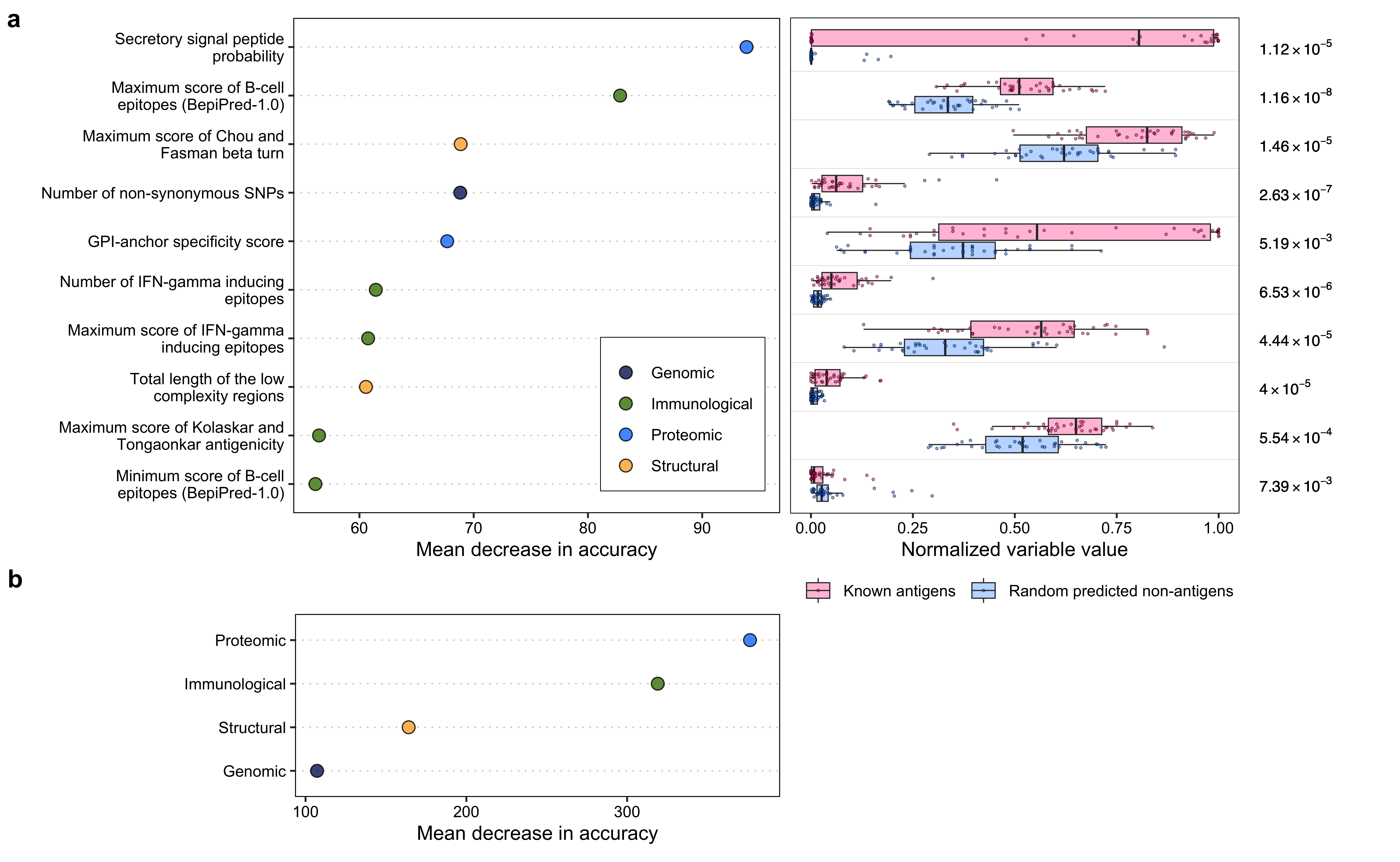

5.4.2.2 Pv + Pf combined data set

# Variable importance
var_imp <- read.csv("./other_data/pfpv_known_antigen_variable_importance.csv")
var_imp <- var_imp[order(-var_imp$meanDecreaseAccuracy), ]
var_imp <- var_imp[1:10, ]

metadata <- read.csv("./data/supplementary_data_1_protein_variable_metadata.csv", check.names = FALSE)
metadata <- metadata[c("category", "column name")]
metadata <- metadata[metadata$`column name` %in% var_imp$variable, ]

var_imp <- merge(x = var_imp, y = metadata, by.x = "variable", by.y = "column name")
var_imp$category <- factor(var_imp$category, levels = names(colorset))
var_imp$color <- sapply(var_imp$category, function(x) colorset[x])

var_imp$variable_ <- c(
  "Percentage of aspartic acid\n minus percentage of glutamic acid",
  "GPI-anchor specificity score",
  "Total length of the low\n complexity regions",
  "Maximum score of Parker\n hydrophilicity",
  "Number of non-synonymous SNPs",
  "Percentage of amino acids with\n normalized van der Waals volume\n between 4.03–8.08",
  "Number of IFN-gamma inducing\n epitopes",
  "Percentage of amino acids with\n polarizability between 0.219–0.409",
  "Small amino acid percentage",
  "Secretory signal peptide\n probability"
)

p1 <- ggplot(var_imp, aes(x = reorder(variable_, meanDecreaseAccuracy), y = meanDecreaseAccuracy, fill = category)) +
  geom_point(size = 3, pch = 21, color = "black", alpha = 0.8) +
  scale_fill_manual(values = colorset, labels = c("Genomic", "Immunological", "Proteomic", "Structural")) +
  coord_flip() +
  ylim(min(var_imp$meanDecreaseAccuracy), max(var_imp$meanDecreaseAccuracy) + 1) +
  theme_bw() +
  theme(
    panel.grid.major = element_blank(),
    panel.grid.minor = element_blank(),
    panel.grid.major.y = element_line(color = "grey80", linewidth = 0.3, linetype = "dotted"),
    strip.background = element_blank(),
    panel.border = element_rect(color = "black"),
    legend.text = element_text(color = "black"),
    plot.title = element_text(hjust = 0.5, size = 20),
    plot.margin = ggplot2::margin(10, 10, 0, 10, "pt"),
    axis.title.x = element_text(color = "black"),
    axis.title.y = element_text(color = "black"),
    axis.text.x = element_text(color = "black"),
    axis.text.y = element_text(color = "black"),
    legend.title = element_blank(),
    legend.position = c(0.8, 0.2),
    legend.background = element_rect(colour = "black", linewidth = 0.2)
  ) +
  xlab("") +
  ylab("Mean decrease in accuracy")

# Group variable importance
grp_var_imp <- read.csv("./other_data/pfpv_known_antigen_group_variable_importance.csv")

grp_var_imp_ <- grp_var_imp
firstup <- function(x) {
  substr(x, 1, 1) <- toupper(substr(x, 1, 1))
  return(x)
}
grp_var_imp_$variable <- sapply(grp_var_imp_$variable, function(x) {
  x <- str_replace_all(x, "[_\\.]", " ")
  x <- firstup(x)
  return(x)
})

grp_var_imp_$category <- factor(tolower(grp_var_imp_$variable))

p2 <- ggplot(grp_var_imp_, aes(x = reorder(variable, meanDecreaseAccuracy), y = meanDecreaseAccuracy, fill = category)) +
  geom_point(size = 3, pch = 21, color = "black", alpha = 0.8) +
  scale_fill_manual(values = colorset, labels = c("Genomic", "Immunological", "Proteomic", "Structural")) +
  coord_flip() +
  ylim(min(grp_var_imp$meanDecreaseAccuracy), max(grp_var_imp$meanDecreaseAccuracy) + 5) +
  theme_bw() +
  theme(
    panel.grid.major = element_blank(),
    panel.grid.minor = element_blank(),
    panel.grid.major.y = element_line(color = "grey80", linewidth = 0.3, linetype = "dotted"),
    strip.background = element_blank(),
    panel.border = element_rect(color = "black"),
    legend.text = element_text(color = "black", size = 10),
    plot.title = element_text(hjust = 0.5, size = 20),
    plot.margin = ggplot2::margin(30, 10, 10, 90, "pt"),
    axis.title.x = element_text(color = "black"),
    axis.title.y = element_text(color = "black"),
    axis.text.x = element_text(color = "black"),
    axis.text.y = element_text(color = "black"),
    legend.position = "none"
  ) +
  xlab("") +
  ylab("Mean decrease in accuracy")

# Wilcoxon text
load(file = "./rdata/pfpv_known_antigen_wilcox_data.RData")
wilcox_res <- read.csv("./other_data/pfpv_known_antigen_wilcox_res.csv")
wilcox_data <- data
wilcox_data$compared_group <- compared_group
wilcox_data <- wilcox_data[wilcox_data$compared_group != -1, ]
wilcox_data <- melt(wilcox_data, id = c("compared_group"))
wilcox_data <- merge(x = wilcox_data, y = merge(x = var_imp, y = wilcox_res), by = "variable", all.y = TRUE)
wilcox_data$tile_pos <- rep(0, nrow(wilcox_data))
wilcox_data$compared_group <- factor(wilcox_data$compared_group)

wilcox_data$variable <- sapply(wilcox_data$variable, function(x) {
  x <- str_replace_all(x, "[_\\.]", " ")
  x <- firstup(x)
  return(x)
})

adj_pval_tmp <- c()
for (i in 1:nrow(wilcox_data)) {
  x <- wilcox_data$adj_pval[i]
  a <- strsplit(format(x, scientific = TRUE, digits = 3), "e")[[1]]
  res <- paste0(sprintf("%0.2f", as.numeric(a[1])), " %*% 10^", as.integer(a[2]))
  adj_pval_tmp <- c(adj_pval_tmp, res)
}
wilcox_data$adj_pval <- adj_pval_tmp

p3 <- ggplot(wilcox_data, aes(x = reorder(variable, meanDecreaseAccuracy), y = value, fill = compared_group)) +
  geom_boxplot(outlier.color = NA, alpha = 0.3, lwd = 0.3) +
  geom_point(
    color = "black", shape = 21, stroke = 0.3, alpha = 0.5, size = 0.5,
    position = position_jitterdodge()
  ) +
  geom_text(aes(label = adj_pval),
    y = 1.1, size = 3, fontface = "plain", family = "sans",
    hjust = 0, parse = TRUE
  ) +
  geom_vline(xintercept = 1:9 + 0.5, color = "grey80", linetype = "solid", linewidth = 0.1) +
  coord_flip(ylim = c(0, 1), clip = "off") +
  scale_fill_manual(
    breaks = c("1", "0"), values = c("#FF007F", "#0080FF"),
    labels = c("Known antigens", "Random predicted non-antigens")
  ) +
  theme_bw() +
  theme(
    panel.grid.major = element_blank(),
    panel.grid.minor = element_blank(),
    strip.background = element_blank(),
    panel.border = element_rect(linewidth = 0.2, colour = "black"),
    plot.title = element_text(hjust = 0.5),
    plot.margin = ggplot2::margin(10, 90, 0, -20, "pt"),
    legend.text = element_text(colour = "black"),
    axis.title.x = element_text(color = "black"),
    axis.title.y = element_text(color = "black"),
    axis.text.x = element_text(color = "black"),
    axis.text.y = element_blank(),
    axis.ticks.y = element_blank(),
    legend.position = "none"
  ) +
  xlab("") +
  ylab("Normalized variable value")

legend <- get_legend(p3 +
  theme(
    legend.title = element_blank(),
    legend.background = element_blank(),
    legend.key = element_blank(),
    legend.direction = "horizontal",
    legend.position = c(0.35, 0.9)
  ))

p_combined <- plot_grid(plot_grid(p1, p3, labels = c("a", ""), rel_widths = c(0.57, 0.43)),
  plot_grid(p2, NULL, legend,
    labels = c("b", "", "", ""),
    nrow = 1, rel_widths = c(0.57, 0.01, 0.42)
  ),
  ncol = 1, rel_heights = c(0.65, 0.35)
)
p_combined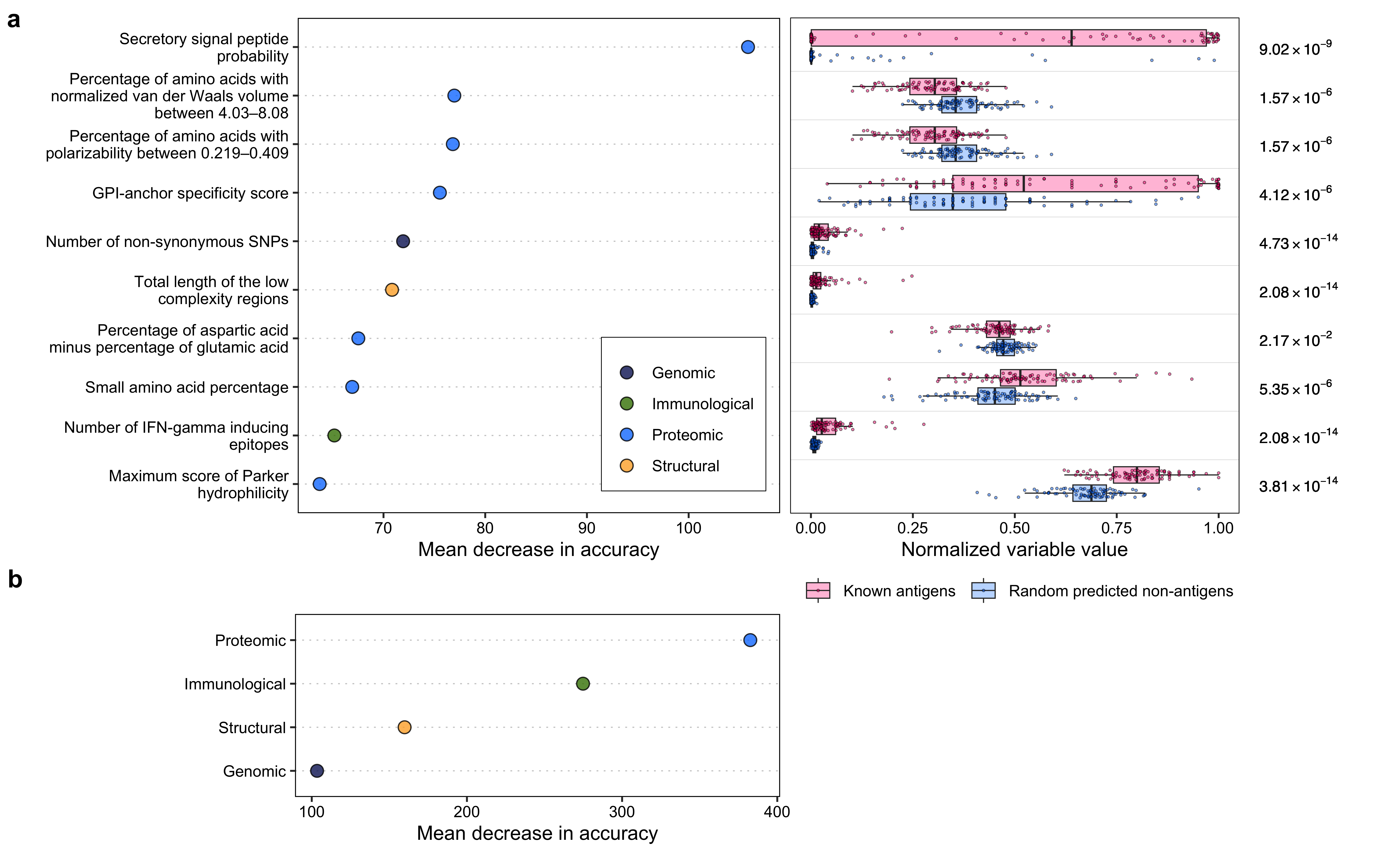

5.4.3 Comparison of top 10 important variables

5.4.3.1 Venn diagram

5.4.3.2 Top 10 variables from combined model

In R

library(ggrepel)

data <- read.csv("./other_data/pfpv_top_10_imp_vars.csv")
data$variable <- c(
  "Secretory signal peptide\n probability",
  "Percentage of amino acids with\n normalized van der Waals volume\n between 4.03–8.08",
  "Percentage of amino acids with\n polarizability between 0.219–0.409",
  "GPI-anchor specificity score",
  "Number of non-synonymous SNPs",
  "Total length of the low\n complexity regions",
  "Percentage of aspartic acid\n minus percentage of glutamic acid",
  "Small amino acid percentage",
  "Number of IFN-gamma inducing\n epitopes",
  "Maximum score of Parker\n hydrophilicity"
)

p1 <- ggplot(data, aes(x = pf_single_model, y = pfpv_combined_model, label = variable)) +
  geom_abline(intercept = 0, slope = 1, alpha = 0.3) +
  geom_point() +
  geom_text_repel(
    size = 2.5, point.padding = 0, min.segment.length = 0,
    max.time = 1, max.iter = 1e5, seed = 42, box.padding = 0.3,
    segment.color = "grey30", segment.size = 0.2, lineheight = 1
  ) +
  theme_bw() +
  theme(
    panel.grid.major = element_blank(),
    panel.grid.minor = element_blank(),
    strip.background = element_blank(),
    panel.border = element_rect(linewidth = 0.2, colour = "black"),
    plot.title = element_text(hjust = 0.5),
    plot.margin = ggplot2::margin(5, 0, 0, 5, "pt"),
    legend.text = element_text(colour = "black"),
    axis.title.x = element_blank(),
    axis.title.y = element_text(color = "black"),
    axis.text.x = element_blank(),
    axis.text.y = element_text(color = "black"),
    axis.ticks.x = element_blank(),
    legend.position = "none"
  ) +
  ylab("Combined model") +
  xlim(0, 110) +
  ylim(0, 110)

p2 <- ggplot(data, aes(x = pv_single_model, y = pfpv_combined_model, label = variable)) +
  geom_abline(intercept = 0, slope = 1, alpha = 0.3) +
  geom_point() +
  geom_text_repel(
    size = 2.5, point.padding = 0, min.segment.length = 0,
    max.time = 1, max.iter = 1e5, seed = 42, box.padding = 0.3,
    segment.color = "grey30", segment.size = 0.2, lineheight = 1
  ) +
  theme_bw() +
  theme(
    panel.grid.major = element_blank(),
    panel.grid.minor = element_blank(),
    strip.background = element_blank(),
    panel.border = element_rect(linewidth = 0.2, colour = "black"),
    plot.title = element_text(hjust = 0.5),
    plot.margin = ggplot2::margin(5, 5, 0, 0, "pt"),
    legend.text = element_text(colour = "black"),
    axis.title.x = element_text(color = "black"),
    axis.title.y = element_blank(),
    axis.text.x = element_text(color = "black"),
    axis.text.y = element_blank(),
    axis.ticks.y = element_blank(),
    legend.position = "none"
  ) +
  xlab(expression(paste(italic("P. vivax"), " model"))) +
  xlim(0, 110) +
  ylim(0, 110)

p3 <- ggplot(data, aes(x = pf_single_model, y = pv_single_model, label = variable)) +
  geom_abline(intercept = 0, slope = 1, alpha = 0.3) +
  geom_point() +
  geom_text_repel(
    size = 2.5, point.padding = 0, min.segment.length = 0,
    max.time = 1, max.iter = 1e5, seed = 42, box.padding = 0.3,
    segment.color = "grey30", segment.size = 0.2, lineheight = 1
  ) +
  theme_bw() +
  theme(
    panel.grid.major = element_blank(),
    panel.grid.minor = element_blank(),
    strip.background = element_blank(),
    panel.border = element_rect(linewidth = 0.2, colour = "black"),
    plot.title = element_text(hjust = 0.5),
    plot.margin = ggplot2::margin(0, 0, 5, 5, "pt"),
    legend.text = element_text(colour = "black"),
    axis.title.x = element_text(color = "black"),
    axis.title.y = element_text(color = "black"),
    axis.text.x = element_text(color = "black"),
    axis.text.y = element_text(color = "black"),
    legend.position = "none"
  ) +
  xlab(expression(paste(italic("P. falciparum"), " model"))) +
  ylab(expression(paste(italic("P. vivax"), " model"))) +
  xlim(0, 110) +
  ylim(0, 110)

p_combined <- plot_grid(plot_grid(p1, p3, ncol = 1),
  plot_grid(p2, NULL, ncol = 1, rel_heights = c(0.53, 0.47)),
  ncol = 2
)
p_combined

sessionInfo()

## R version 4.2.3 (2023-03-15)
## Platform: x86_64-apple-darwin17.0 (64-bit)
## Running under: macOS Big Sur ... 10.16
## 
## Matrix products: default
## BLAS:   /Library/Frameworks/R.framework/Versions/4.2/Resources/lib/libRblas.0.dylib
## LAPACK: /Library/Frameworks/R.framework/Versions/4.2/Resources/lib/libRlapack.dylib
## 
## locale:
## [1] en_US.UTF-8/en_US.UTF-8/en_US.UTF-8/C/en_US.UTF-8/en_US.UTF-8
## 
## attached base packages:
## [1] stats     graphics  grDevices utils     datasets  methods   base     
## 
## other attached packages:
##  [1] stringr_1.5.0     reshape2_1.4.4    rlist_0.4.6.2     rcompanion_2.4.30
##  [5] scales_1.2.1      dendextend_1.17.2 cluster_2.1.4     NbClust_3.0.1    
##  [9] factoextra_1.0.7  DT_0.27           cowplot_1.1.1     ggrepel_0.9.3    
## [13] ggplot2_3.4.2     umap_0.2.10.0     reticulate_1.28  
## 
## loaded via a namespace (and not attached):
##  [1] matrixStats_0.63.0 httr_1.4.6         rprojroot_2.0.3    R.cache_0.16.0    
##  [5] tools_4.2.3        bslib_0.4.2        utf8_1.2.3         R6_2.5.1          
##  [9] nortest_1.0-4      colorspace_2.1-0   withr_2.5.0        tidyselect_1.2.0  
## [13] gridExtra_2.3      Exact_3.2          compiler_4.2.3     cli_3.6.1         
## [17] expm_0.999-7       sandwich_3.0-2     bookdown_0.34      sass_0.4.6        
## [21] lmtest_0.9-40      mvtnorm_1.1-3      proxy_0.4-27       askpass_1.1       
## [25] multcompView_0.1-9 digest_0.6.31      rmarkdown_2.21     R.utils_2.12.2    
## [29] pkgconfig_2.0.3    htmltools_0.5.5    styler_1.9.1       fastmap_1.1.1     
## [33] highr_0.10         htmlwidgets_1.6.2  rlang_1.1.1        readxl_1.4.2      
## [37] rstudioapi_0.14    jquerylib_0.1.4    generics_0.1.3     zoo_1.8-12        
## [41] jsonlite_1.8.4     crosstalk_1.2.0    dplyr_1.1.2        R.oo_1.25.0       
## [45] magrittr_2.0.3     modeltools_0.2-23  Matrix_1.5-4       Rcpp_1.0.10       
## [49] DescTools_0.99.48  munsell_0.5.0      fansi_1.0.4        viridis_0.6.3     
## [53] lifecycle_1.0.3    R.methodsS3_1.8.2  stringi_1.7.12     multcomp_1.4-23   
## [57] yaml_2.3.7         MASS_7.3-60        rootSolve_1.8.2.3  plyr_1.8.8        
## [61] grid_4.2.3         parallel_4.2.3     lmom_2.9           lattice_0.21-8    
## [65] splines_4.2.3      knitr_1.42         pillar_1.9.0       boot_1.3-28.1     
## [69] gld_2.6.6          codetools_0.2-19   stats4_4.2.3       glue_1.6.2        
## [73] evaluate_0.21      data.table_1.14.8  png_0.1-8          vctrs_0.6.2       
## [77] cellranger_1.1.0   gtable_0.3.3       openssl_2.0.6      purrr_1.0.1       
## [81] cachem_1.0.8       xfun_0.39          coin_1.4-2         libcoin_1.0-9     
## [85] e1071_1.7-13       RSpectra_0.16-1    class_7.3-22       survival_3.5-5    
## [89] viridisLite_0.4.2  tibble_3.2.1       ellipsis_0.3.2     TH.data_1.1-2     
## [93] here_1.0.1

session_info.show()

## -----
## Bio                 1.78
## joblib              1.1.1
## numpy               1.19.0
## pandas              1.3.2
## purf                NA
## scipy               1.8.0
## session_info        1.0.0
## sklearn             0.24.2
## -----
## Python 3.8.2 (default, Mar 26 2020, 10:45:18) [Clang 4.0.1 (tags/RELEASE_401/final)]
## macOS-10.16-x86_64-i386-64bit
## -----
## Session information updated at 2023-05-18 12:35